Glenn’s Computer Museum |
| Home | New | Old Military | Later Military | Analog Stuff | IBM Stuff | S/3 Mod 6 | S/32 | Components | Encryption | Misc | B61 |
change log |
contact me |
![]()
Glenn’s Computer Museum |
| Home | New | Old Military | Later Military | Analog Stuff | IBM Stuff | S/3 Mod 6 | S/32 | Components | Encryption | Misc | B61 |
change log |
contact me |
![]()
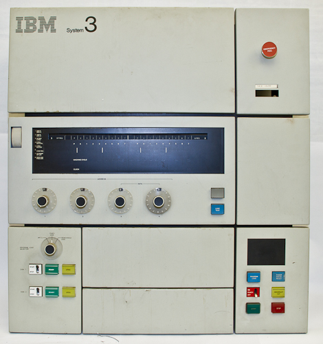


The IBM System/3 family was a very successful line of small business-oriented computers in the 1970's. The first member, the Model 10, shipped in mid-1969 and was a card-based batch-oriented system intended to replace unit-record (punched card) commercial applications: billing, inventory control, accounts receivable, sales analysis, payroll, etc. The System/3 applications were written in RPG, a non-procedural language originally based on the data-flow of IBM card-based accounting machines. Of particular interest, the Model 10 introduced a new format of punched card along with I/O devices for it. This card was much smaller than the standard IBM card but could contain more data: 96 columns vs. 80 columns.
Figures 1 and 2 show our console from the card-oriented IBM System/3 Model 10.
The System/3 Model 6,shipped in late 1970, was the second model introduced. As opposed to the card-based batch-oriented Model 10, the System/3 Model 6 was designed for interactive usage, both for business applications, but also for engineering and scientific applications. It had no attached card equipment, but rather had a good keyboard and an (optional) CRT display. The business applications used the same general operating system and RPG language, but there was a new interactive BASIC-language operating system for engineering and scientific applications.
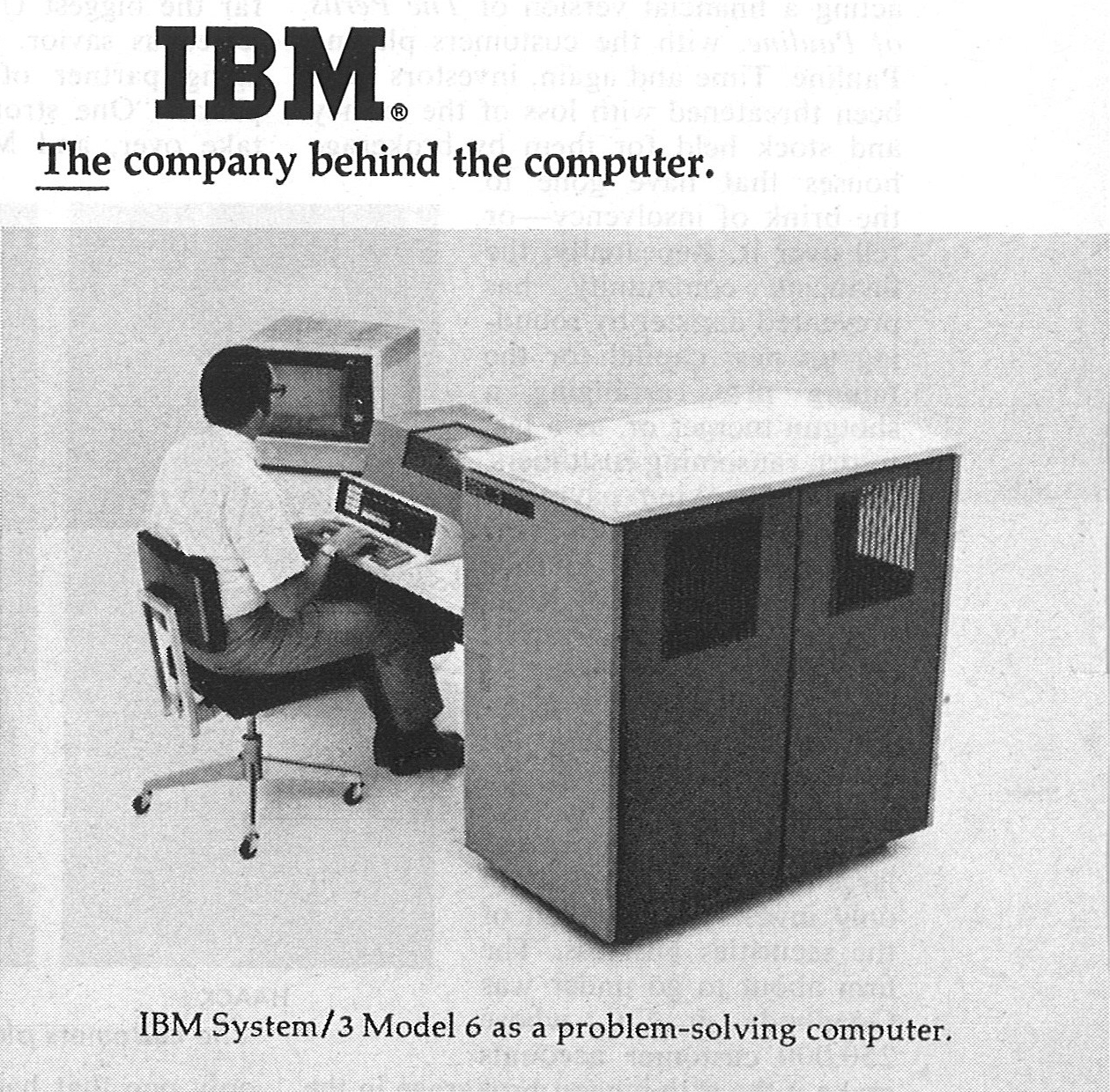
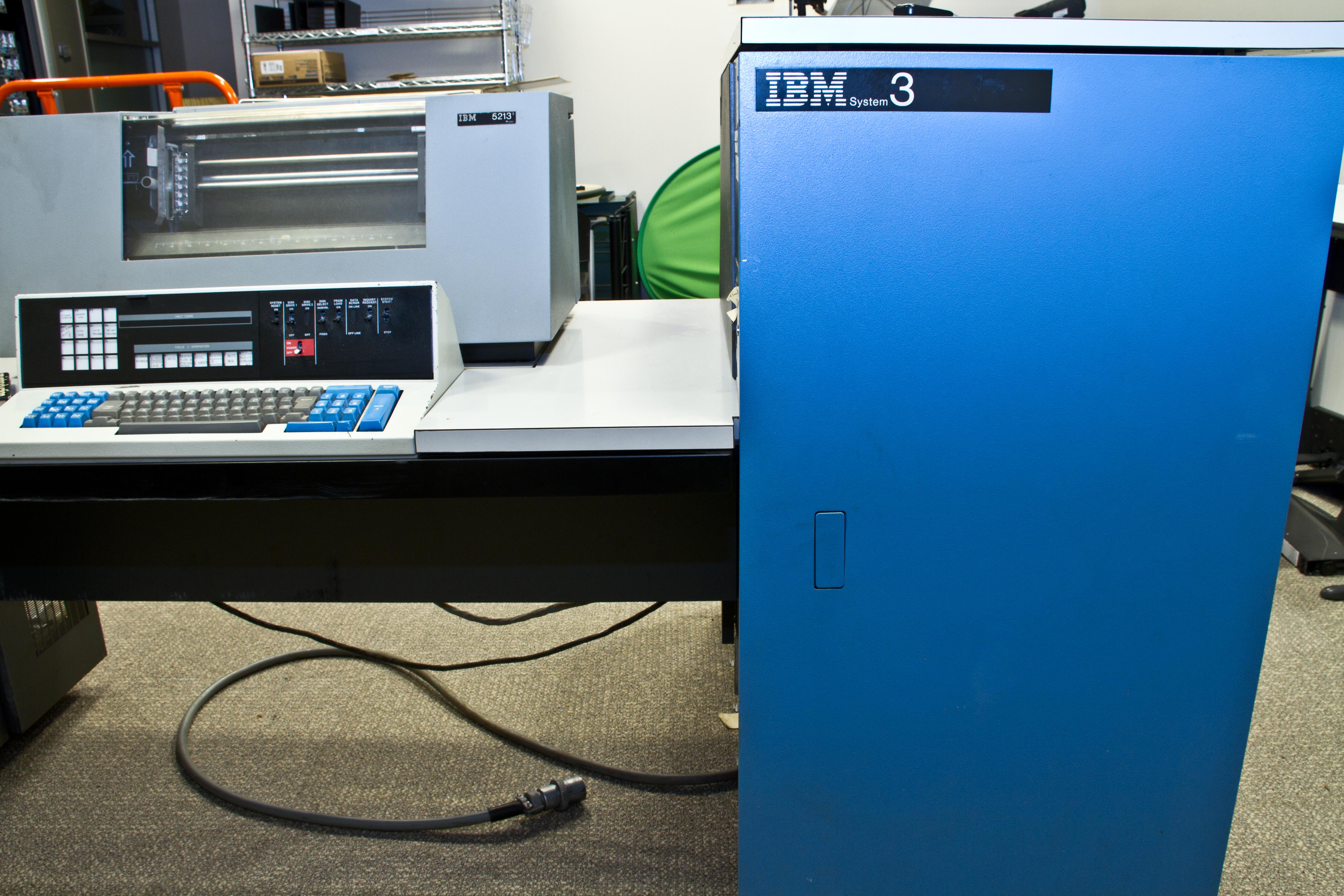
Figure 3, from an IBM ad, shows a person using the System/3 Model 6 with its BASIC software package. Figures 4 etc. show the museum's Model 6 (we do not have the optional CRT display).
In 1968 I was working at IBM San Jose on the design of a follow-on to the IBM 1130, a small engineering and scientific computer. Late in the year, our project was redirected by upper management to use another IBM processor that was being developed in Rochester: the IBM System/3 processor. This was probably the worst architecture ever imagined for engineering and scientific computing:
I was redirected as well--to the newly forming Boca Raton development laboratory. I arrived in Boca in early 1969 and became the manager of one of two departments developing the IBM System/3 Model 6 BASIC program. I managed the operating system underlying the BASIC interpreter. My department implemented a 64KB virtual memory (in software, there was no address translation hardware), the math library, the I/O subsystem, a powerful desk calculator function (ala the later UNIX "bc" function), and an integrated, disk-based help system. In spite of my complaints about the System/3 instruction set, the BASIC system actually performed well.
In addition to the BASIC project being my first IBM management job, I also met my wife while working on this project; she was an IBM programmer in Boca working on operating system development. (In fact, as a nice touch, my System/3 Model 6 arrived literally on the day of our 42th anniversary.)
After my work on the System/3 Model 6 was finished, I worked on the design of another small computer system. That project was cancelled and, in the Fall of 1971, I moved to Rochester where my new job was ss the second-line manager of the system software for another new small computer system: the IBM System/32. Amazingly, the museum also has our own System/32, check it out.
The IBM System/3 Model 6 hardware together with its BASIC software package was, I claim, the first "IBM Personal Computer"; that is, a computer on a desk with a keyboard and a CRT display device, a printer, a removable disk drive, and software for a user to program in interactive BASIC. Effectively, this system could do what the Apple II did, only much better (internal fixed disk, 64KB virtual memory, etc.), and 9 years earlier.
The only flaws with our solution was that it was a large desk with an large lump on one end, it weighed 1,300 lbs, it used 220V power, and it rented for about $1,000 a month. Accordingly, sales were low and the BASIC software received little attention in the market or within IBM. (In spite of the BASIC system having no visibility, I and another person from my department [Brad Beitel] went on to be very successful at IBM.)
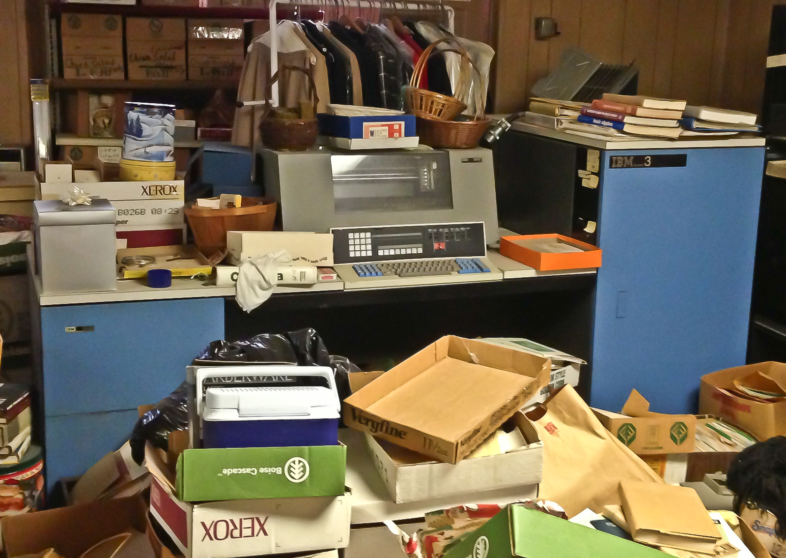
My Model 6 was procured in August, 2013. It came from the original owner who had used it to run business applications for her small company. It was used for this purpose until about 1985 when it was decommissioned by IBM and stored in the owner's basement, where it gradually became buried under typical basement storage items (show in Figure 23).
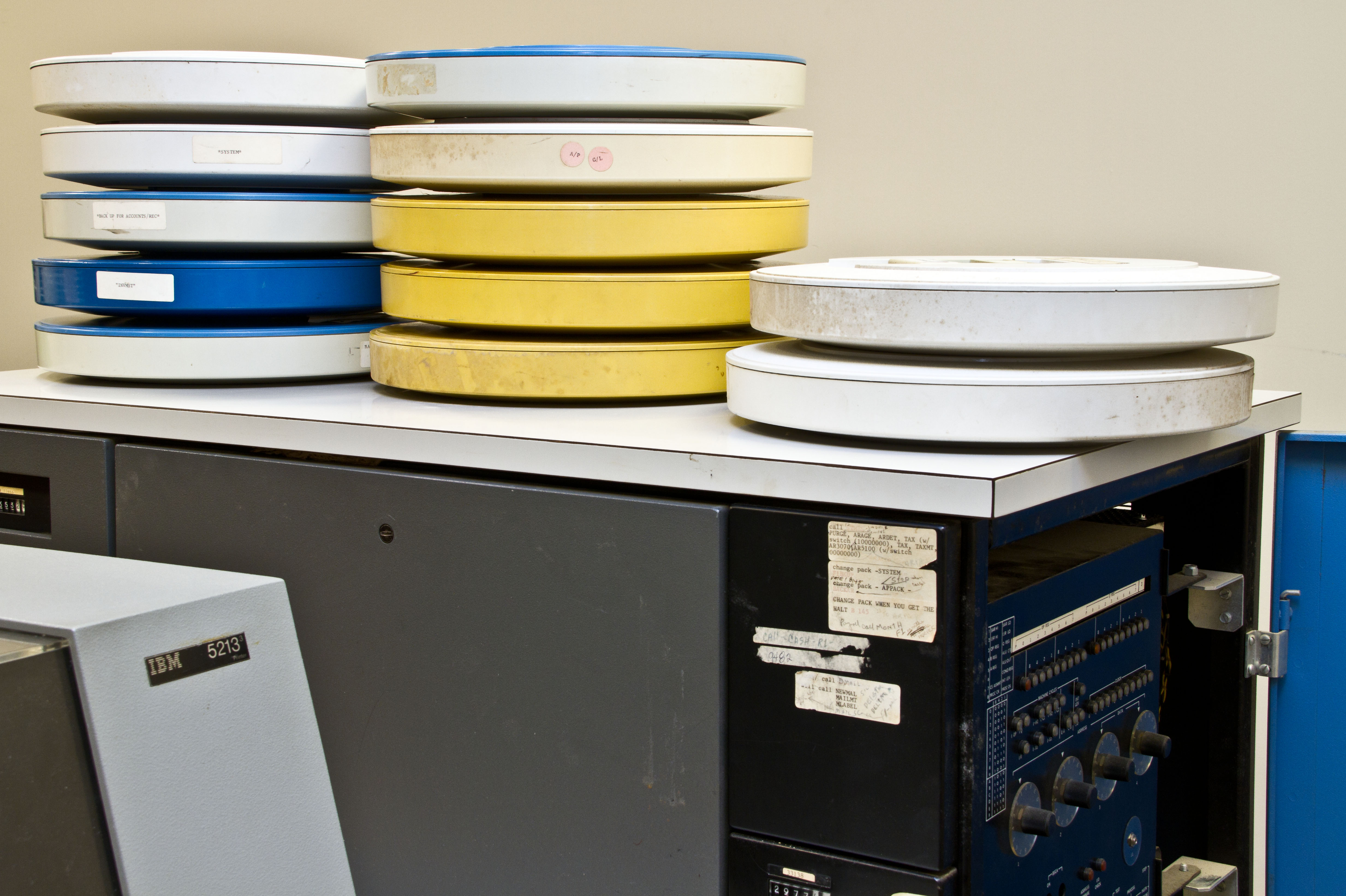
Getting it physically to the museum (in Austin) from the basement in Omaha was a complicated logistically operation, but it finally made it. (Mark Rothbauer of Centaur was the key person here; he went to Omaha and freed it from the basement.) The system's condition is dusty but good considering the it is over 40 years old and hasn't been used for over 25 years. The usage meter indicates 2977 hours powered on. The Model 6 also came with 17 disk packs including the operating system, as well as a lot of documentation.
I (with help from others here at Centaur) will try to restore it to running condition. The likely things that need repairing are replacing electrolytic capacitors and drive belts, but my biggest worry is the disk drive. Stay tuned for progress.
The Model 6 is very rare these days. A interesting web site that covers System/3 family tracks existing devices. It knows of only two other Model 6's, neither of which are operational.
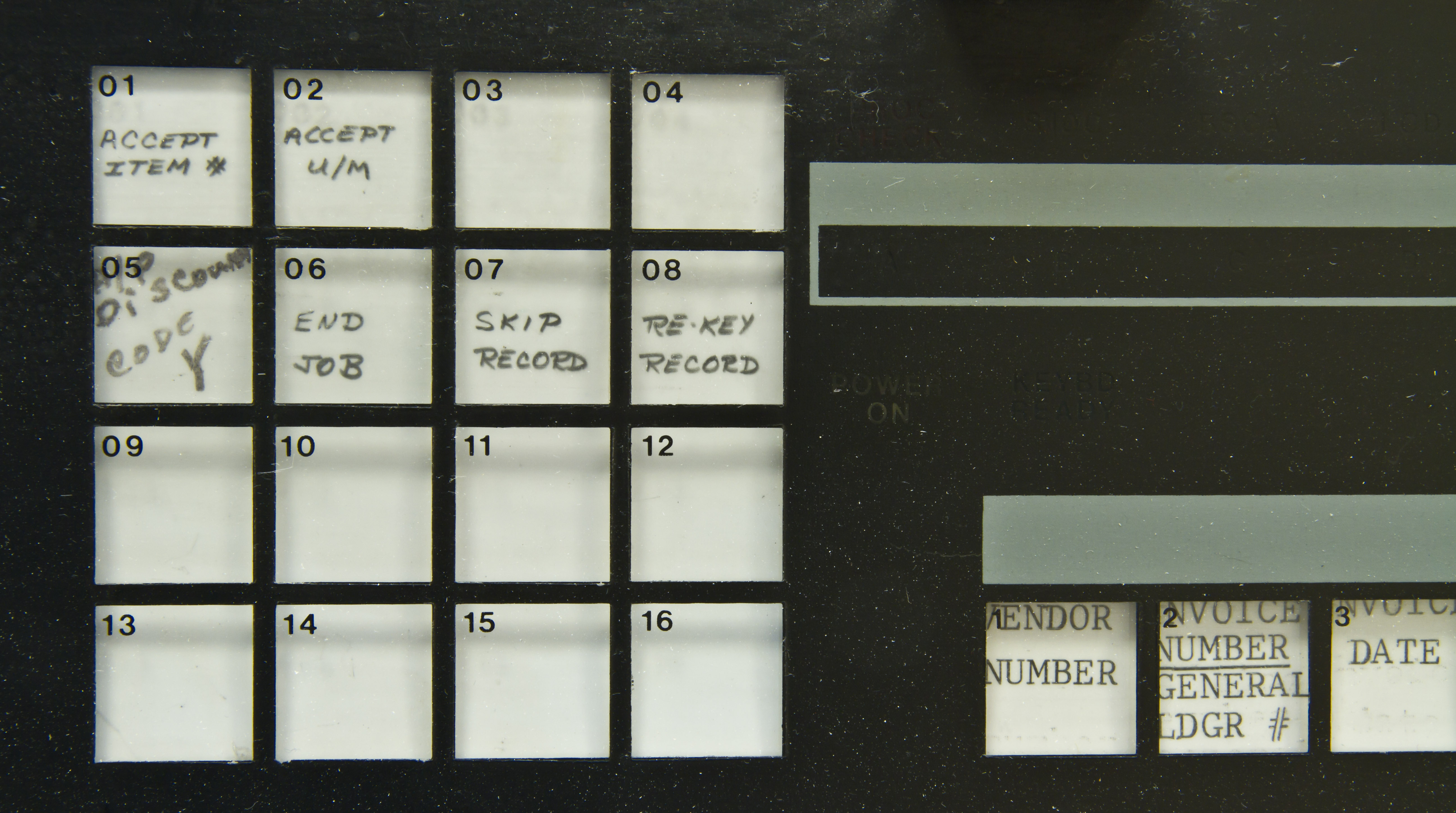
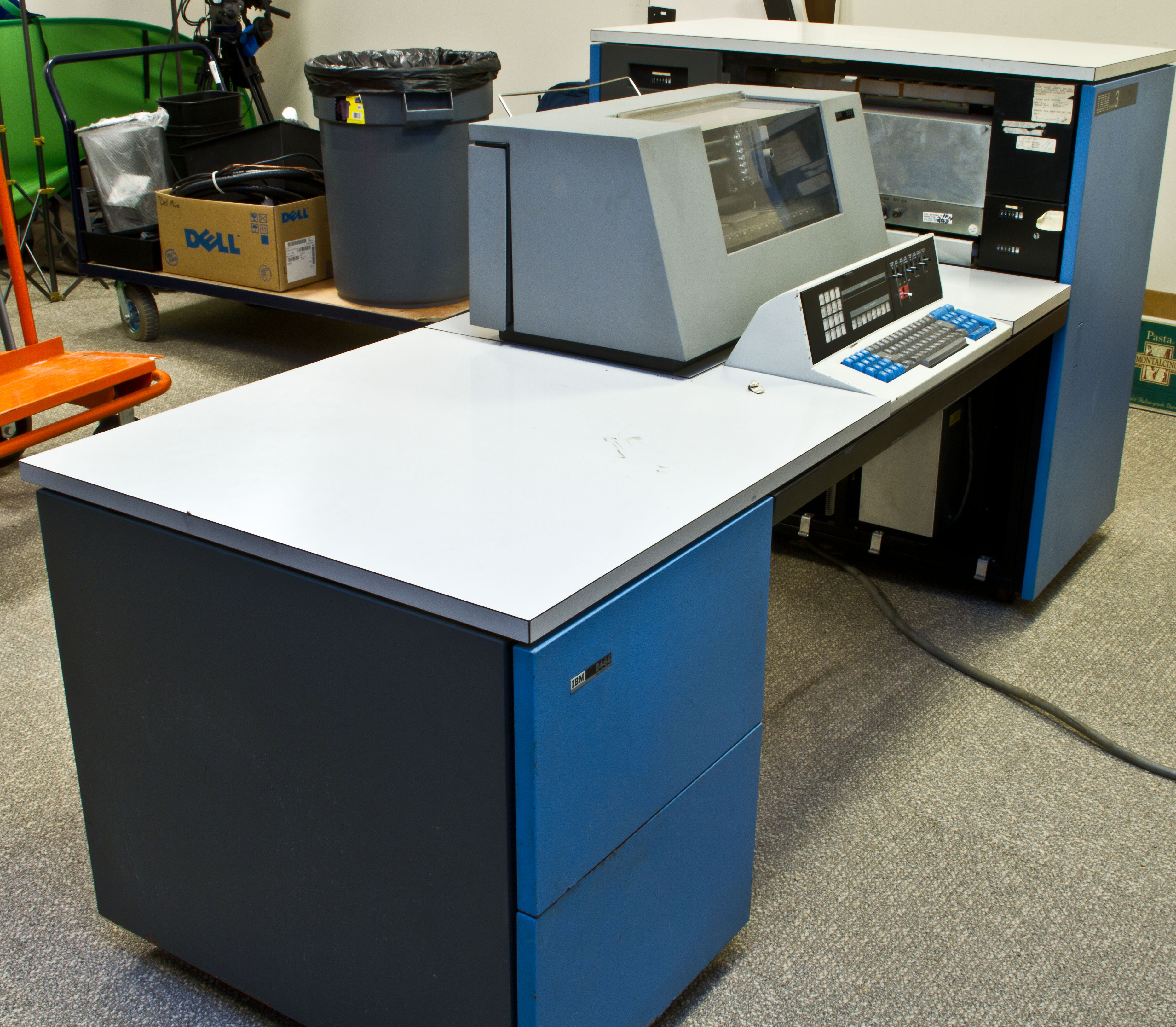
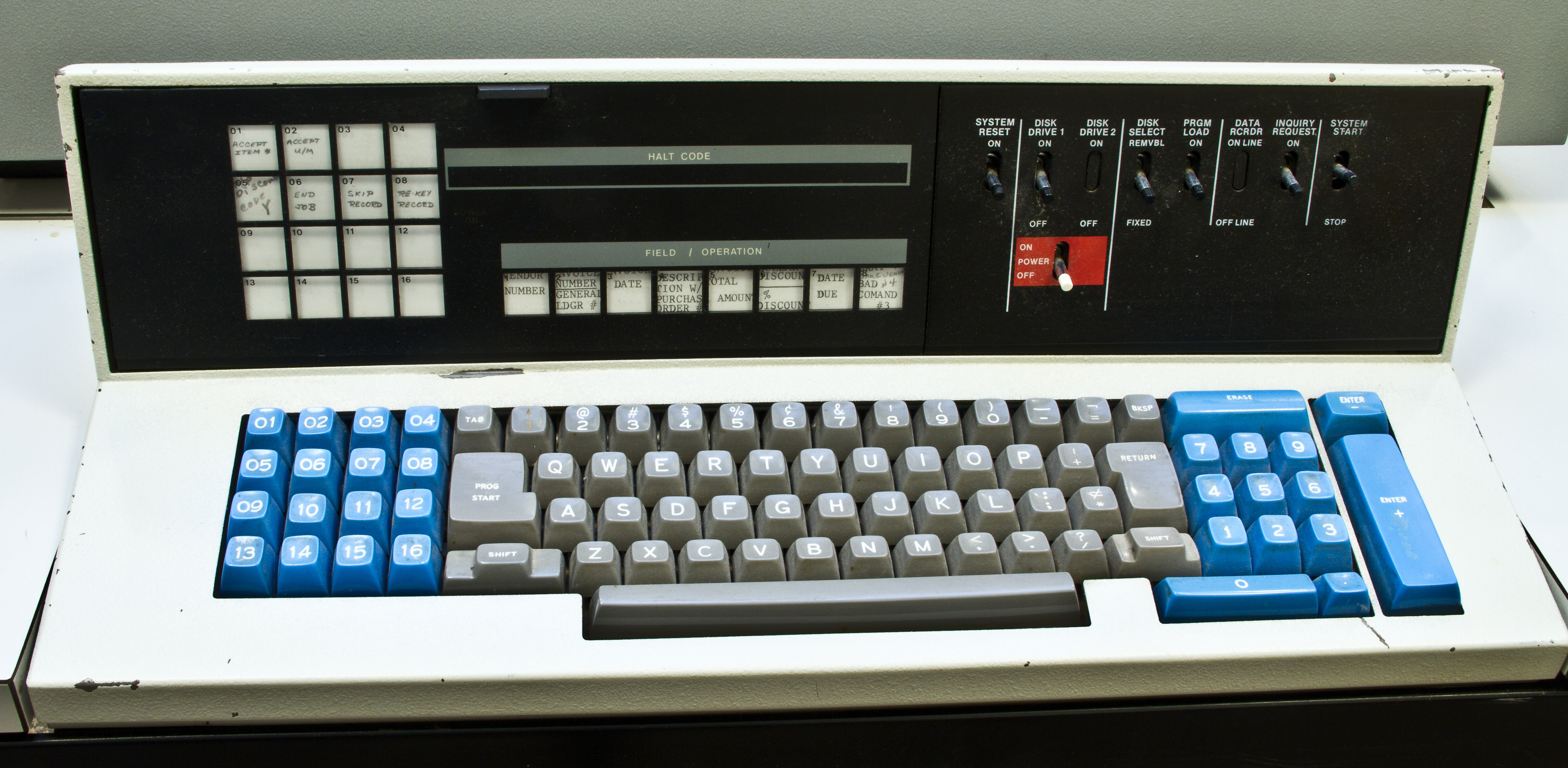
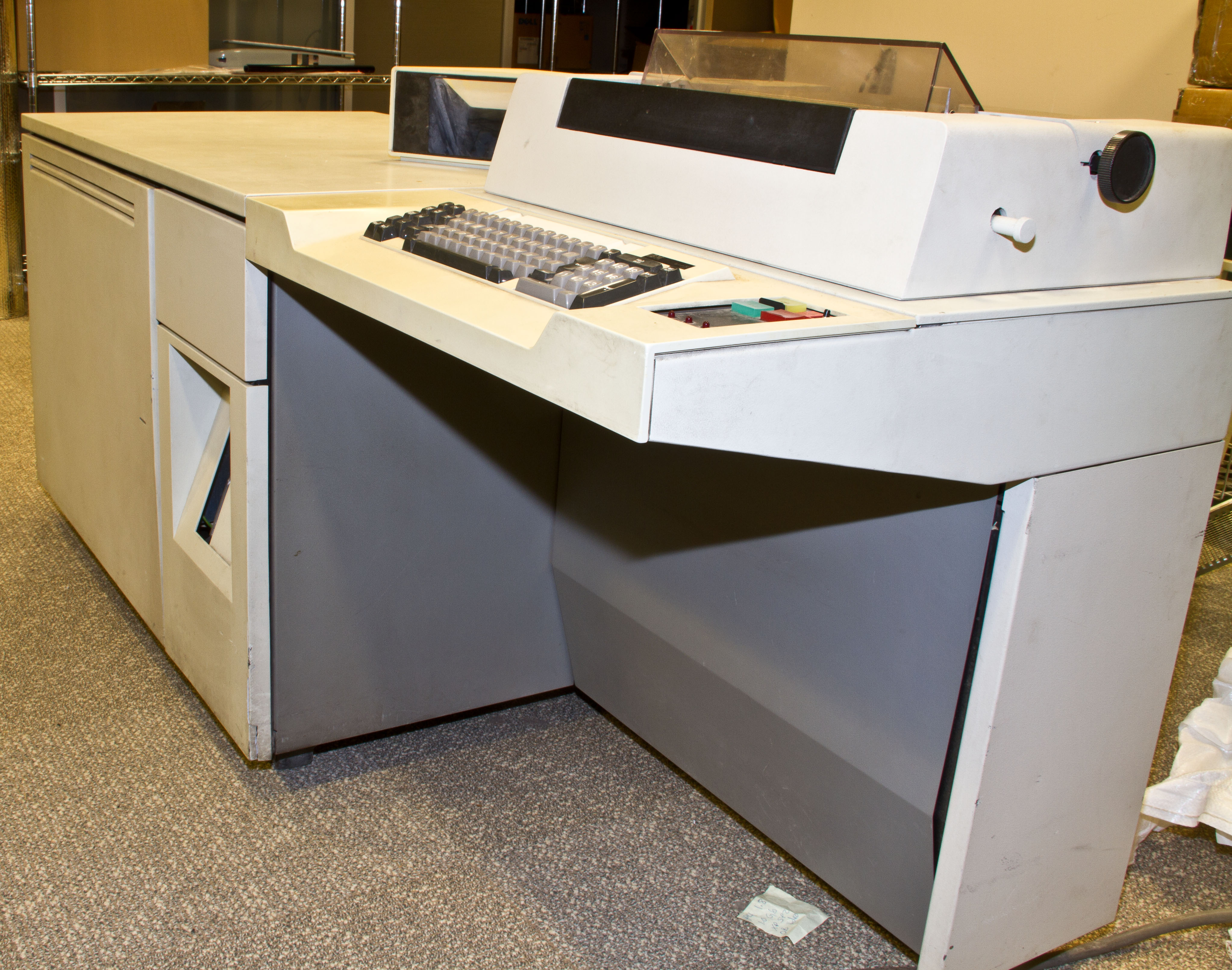
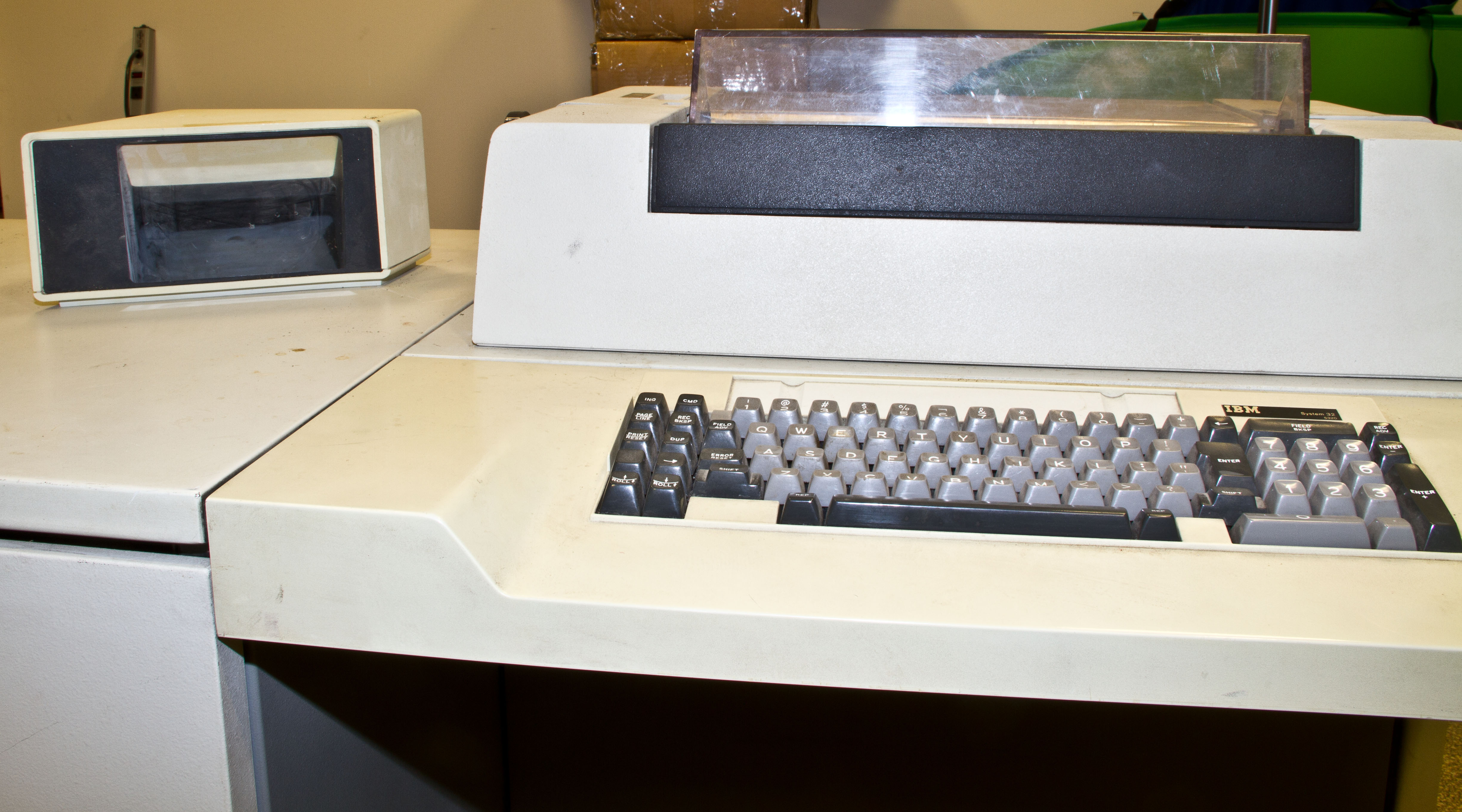
Figures 3, 4, and 5 show the general layout. Figure 6 shows the keyboard, which is very nice, especially for that time. Included are a numerical keypad and 16 function keys. The keyboard complex also included the basic controls for the operator along with "halt code" lights which the program can set. Figure 7 show detail of the 16 lights corresponding to the function keys. These keys are used by the application program and thus have user-writable labels on the lights to remind the operator of what the keys do. To the right of the function key labels there are another eight output lights that can be set by the program. These also have user-writable labels and are used to tell the operator what function to perform next.
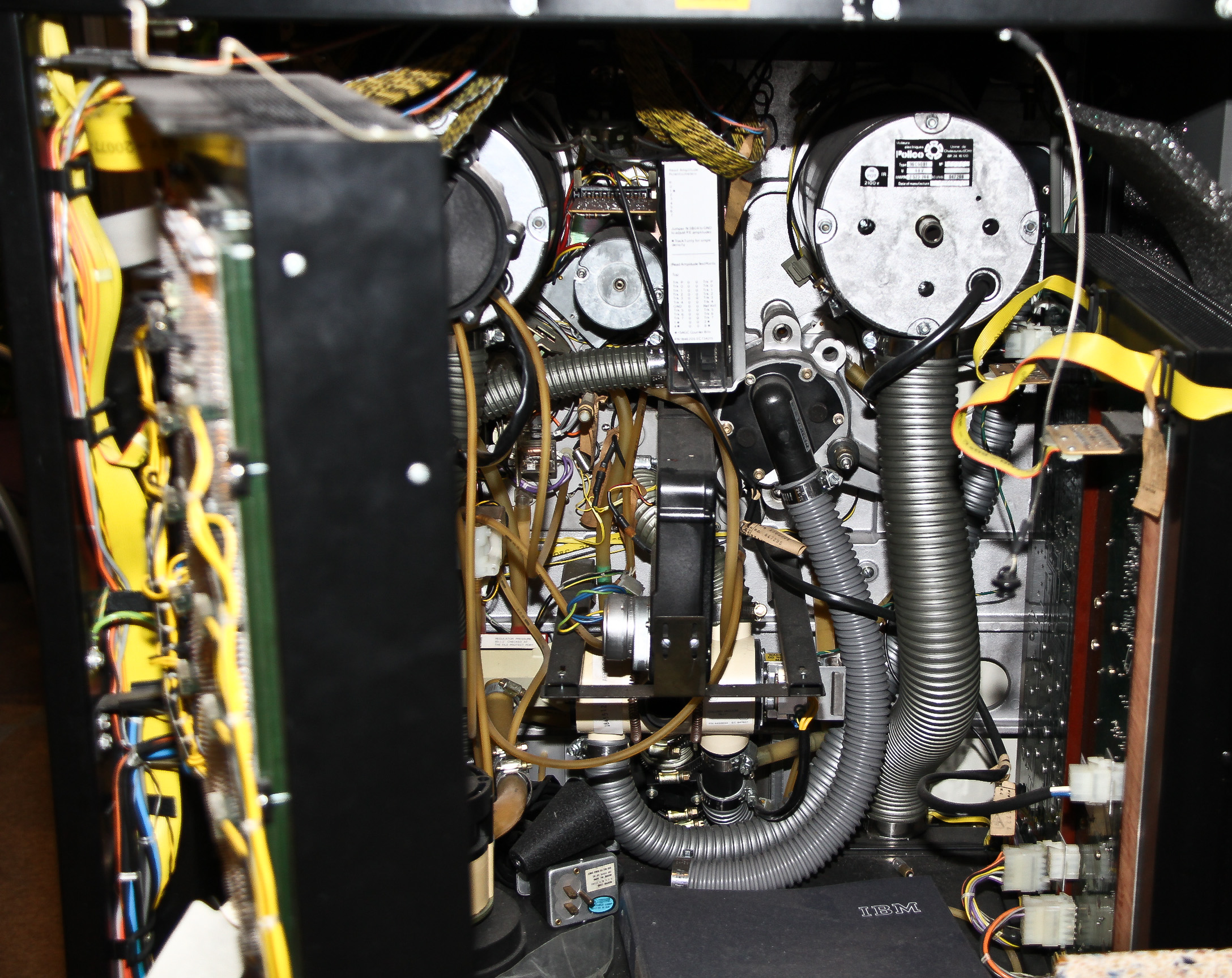
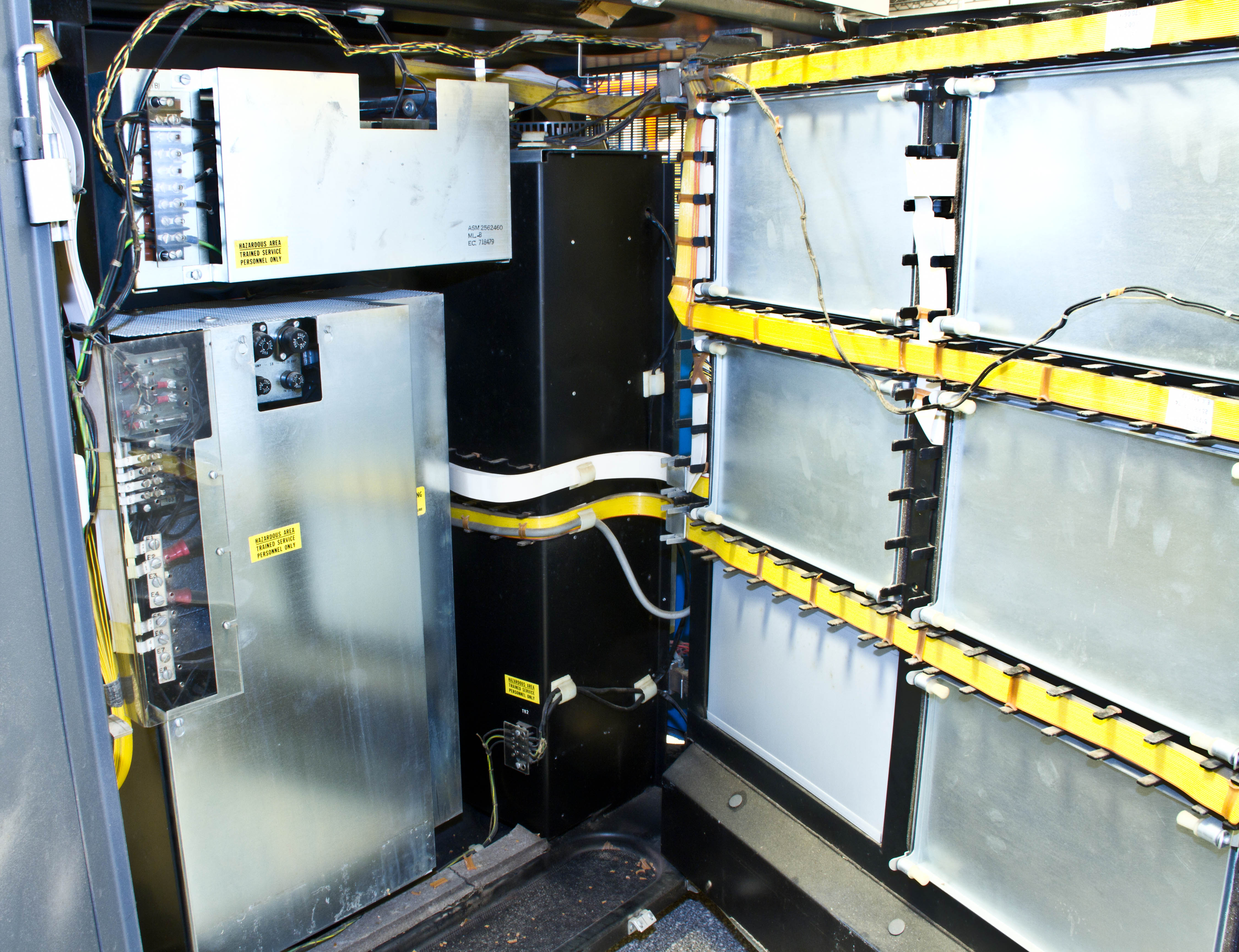
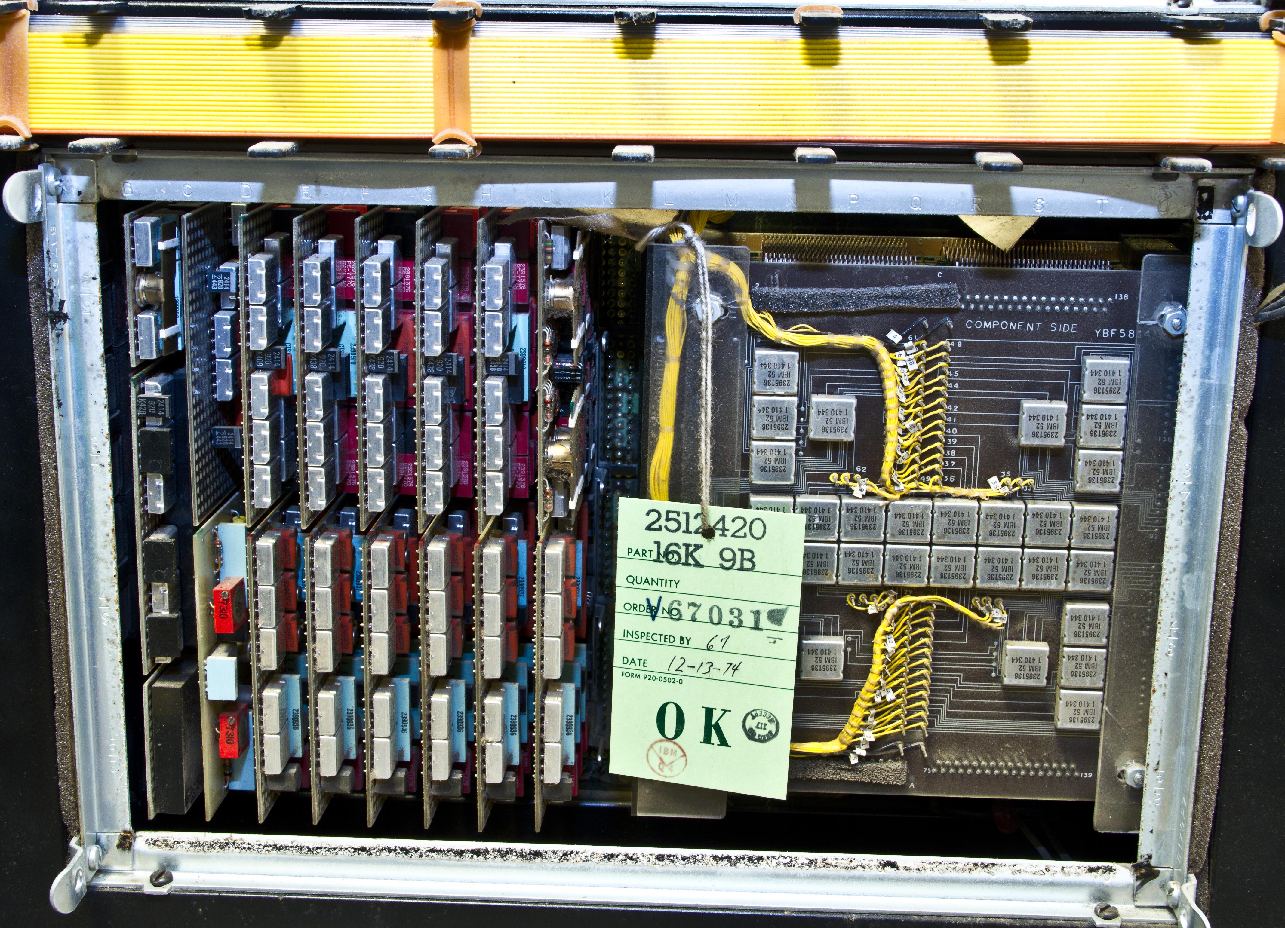
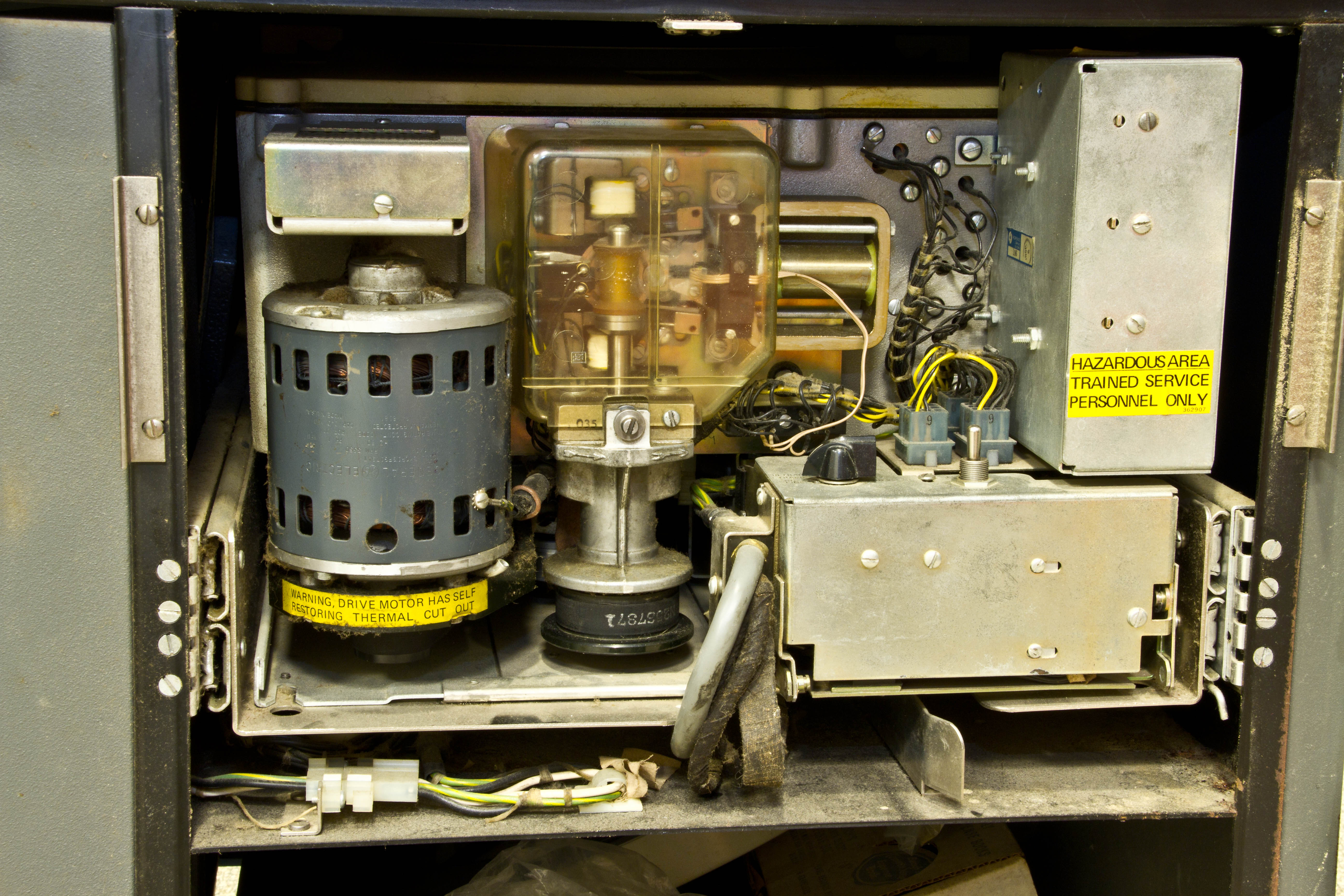
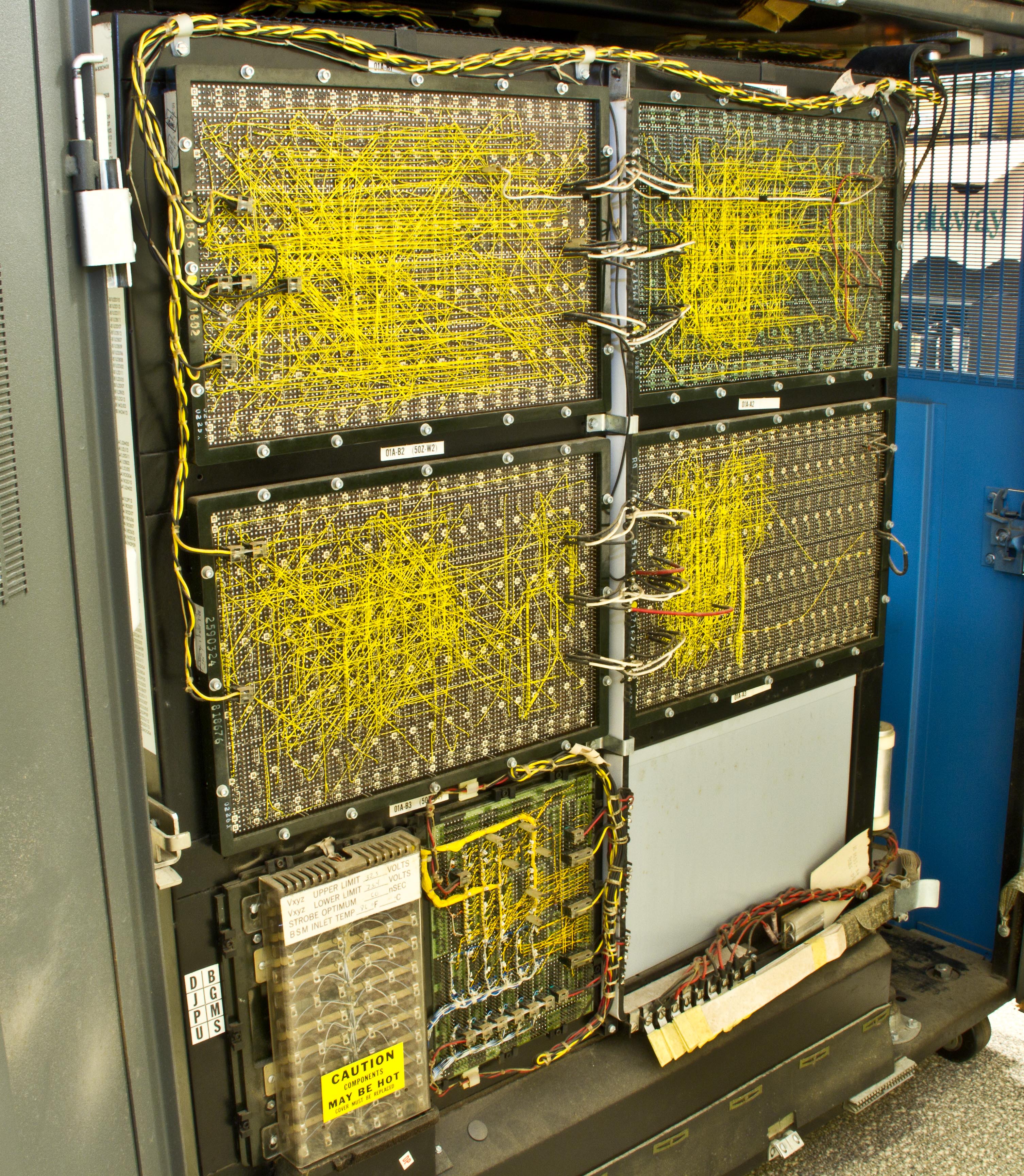
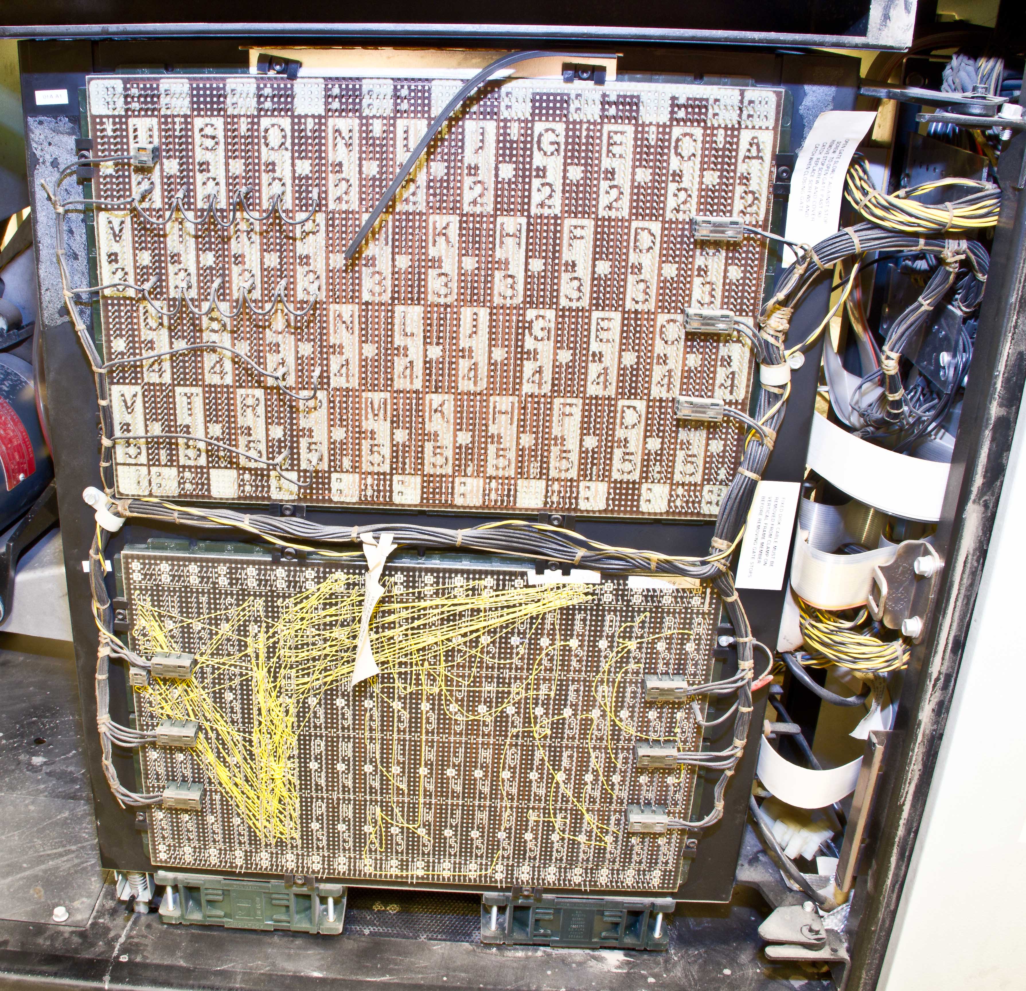
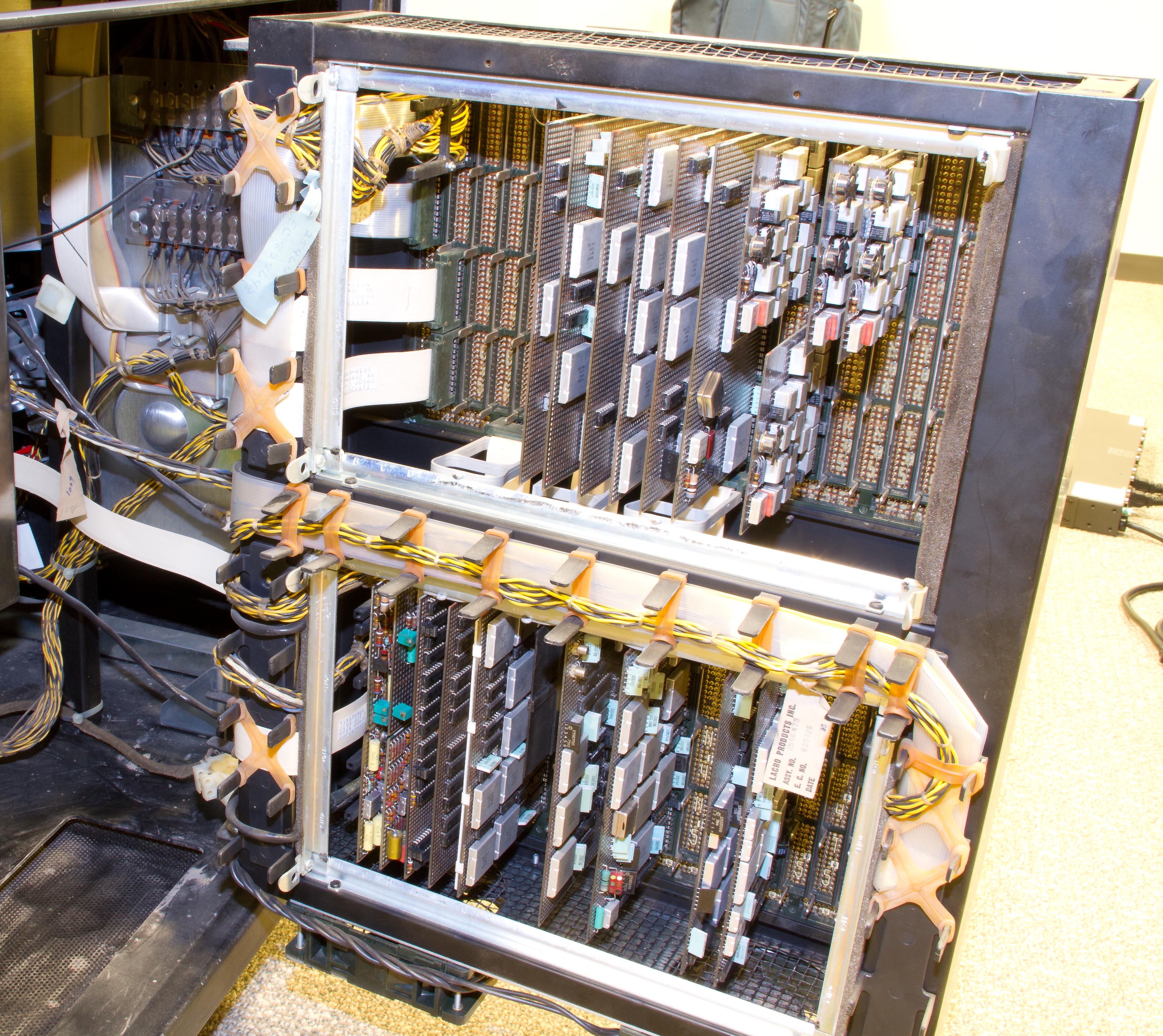
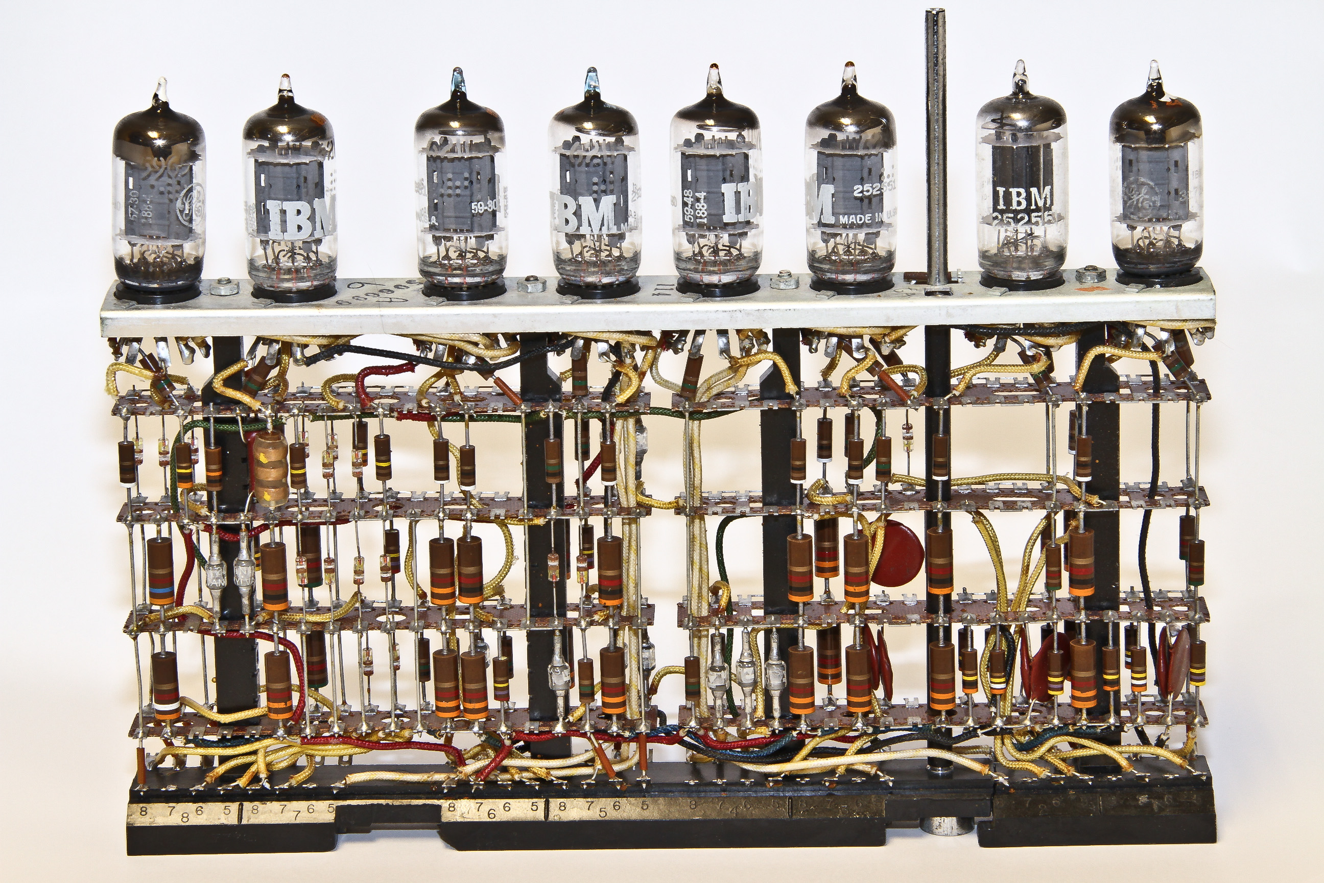
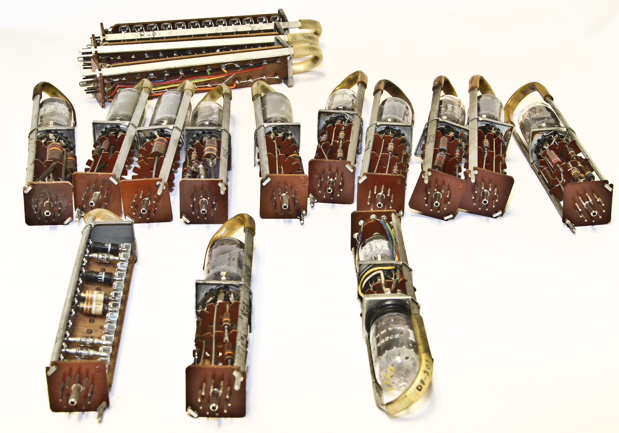
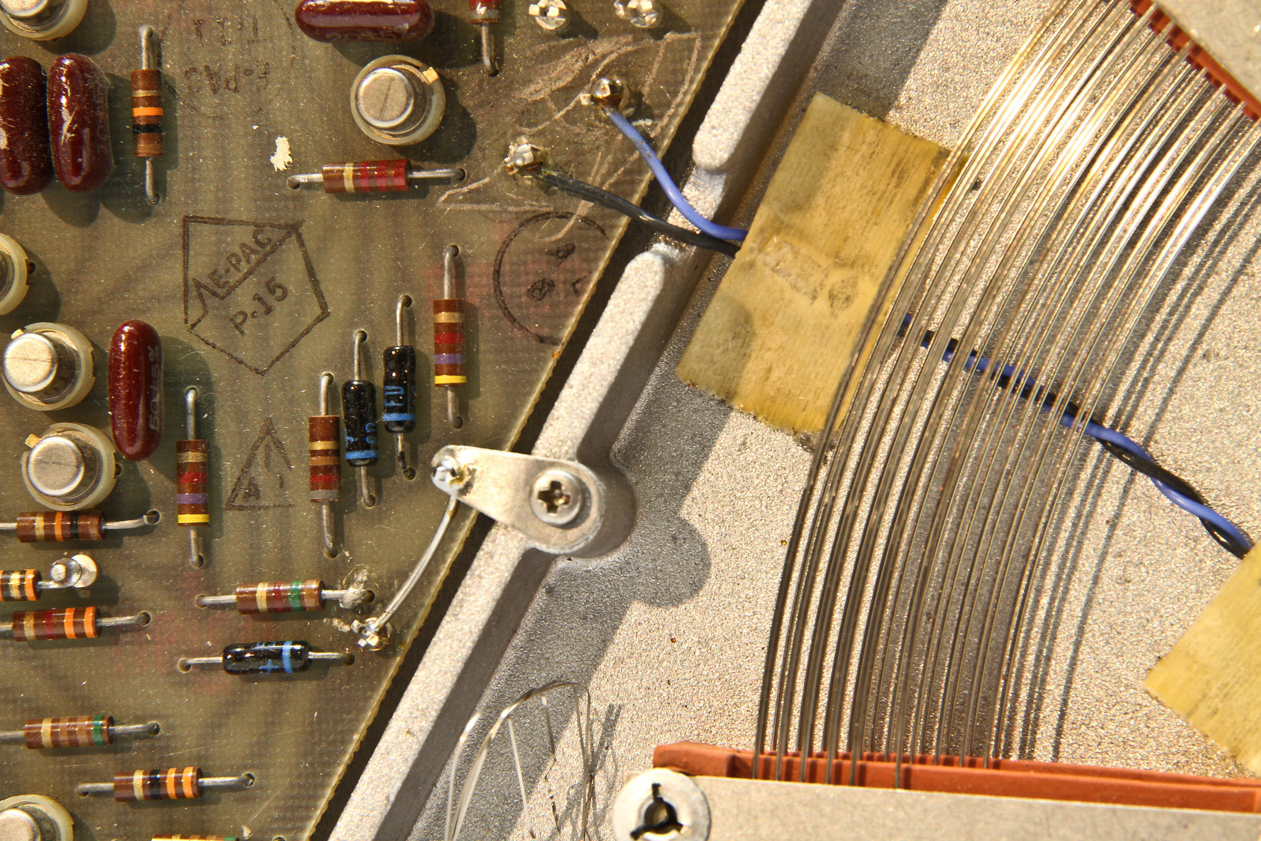
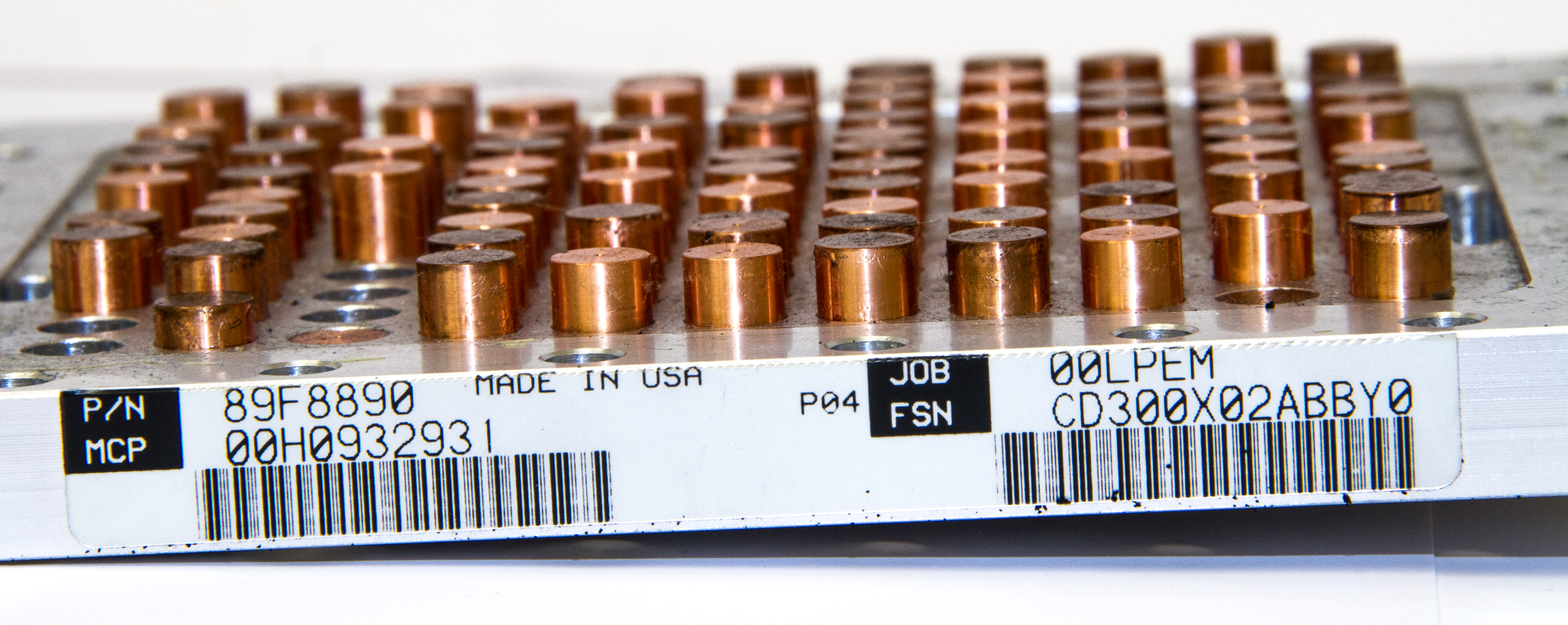
Figure 8 shows the back of the swing-out logic gate with its wiring. There are five logic boards installed. (The missing one is for a communication option). Figure 9 show the other side of the gate and Figure 10 shows it with the board covers removed. Figure 11 shows a closeup of a particularly interesting board. On the left of this board are eight pluggable cards, each containing many modules, primarily IBM MST logic modules (more on this technology below). On the right of this board is the magnetic-core memory module. Our system is fortunate in that it has the largest possible Model 6 memory: 16KB. The smallest memory for a Model 6 was 8KB. (The BASIC software package I worked on ran in only 8KB).
(The Model 6 was probably the last IBM computer to use core memory. Subsequent System/3 models used solid state memory as did the S/370 IBM mainframe family at this time.)
The System/3 instruction set was very simple. It had 28 instructions, two index registers, a condition flags register, and some control registers. There were no accumulator or general purpose registers; operations were performed memory-to-memory. For example, the ALC (Add Logical Characters) instruction (4-6 bytes long, based on addressing options) adds one memory field to another field, one-byte at a time for a specified length from 1 to 256 bytes. Instruction timing is simple: 1.52μs for each memory byte touched. For example, a 4-byte ALC instruction moving 16 bytes in memory takes 30.4μs.
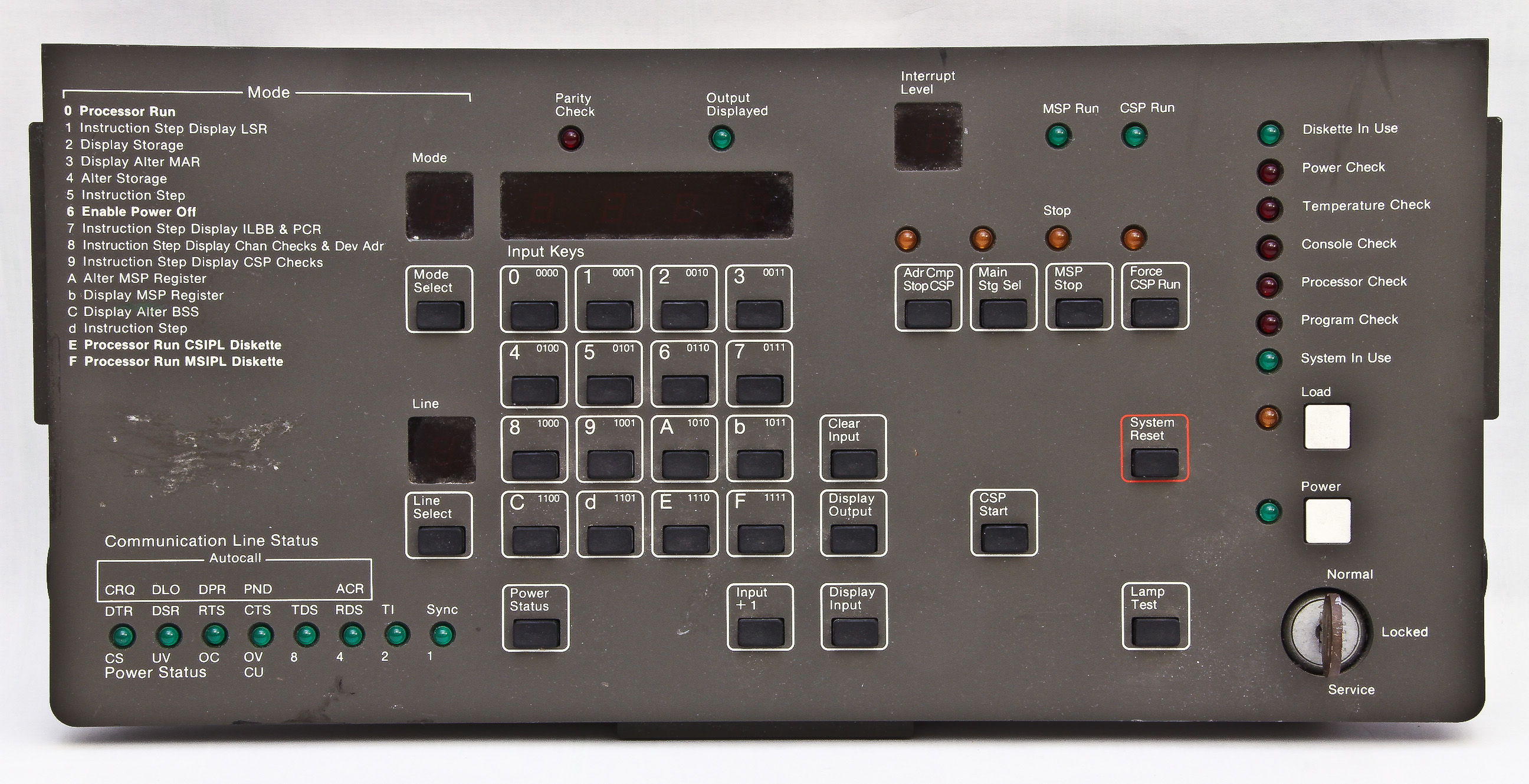
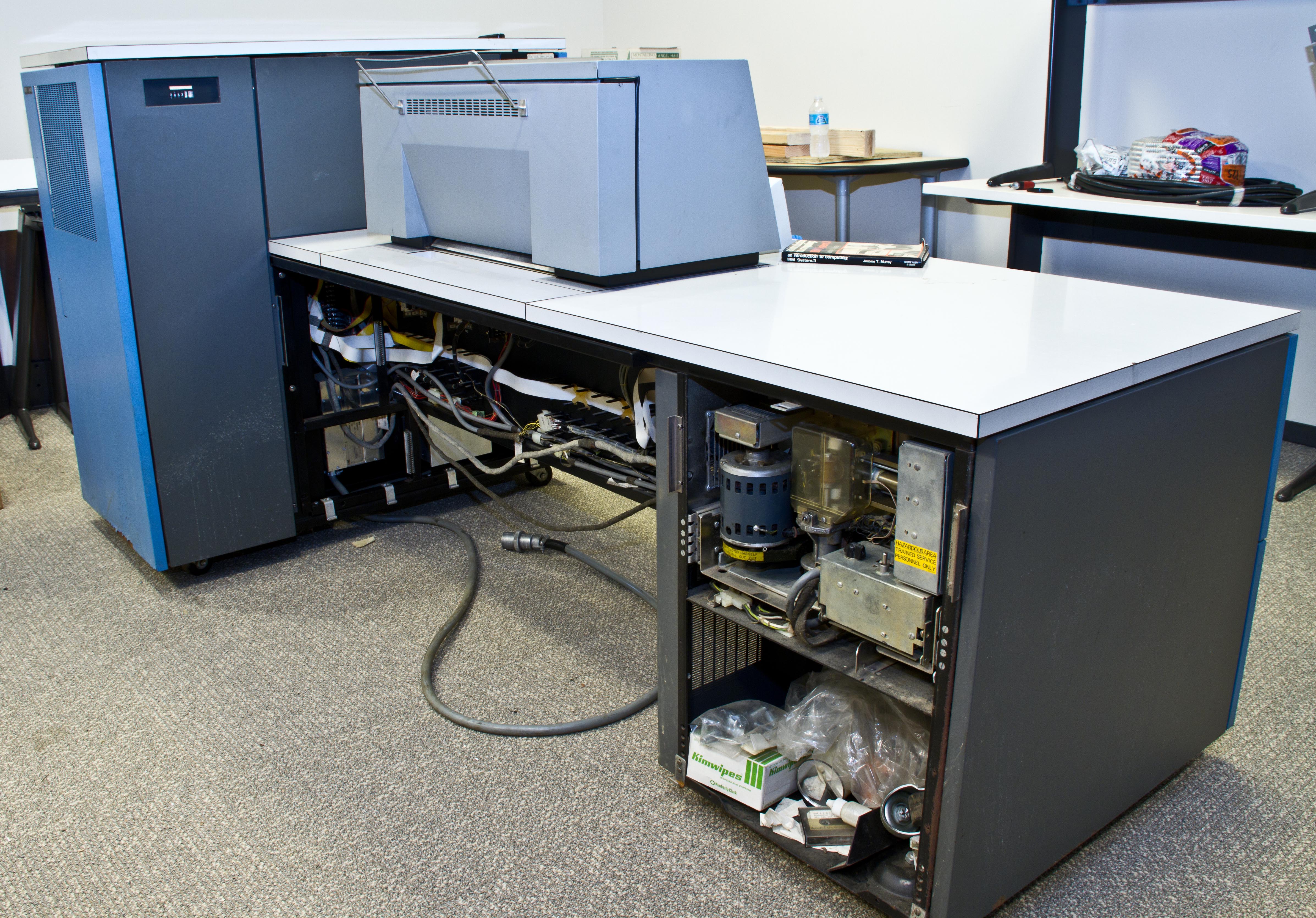
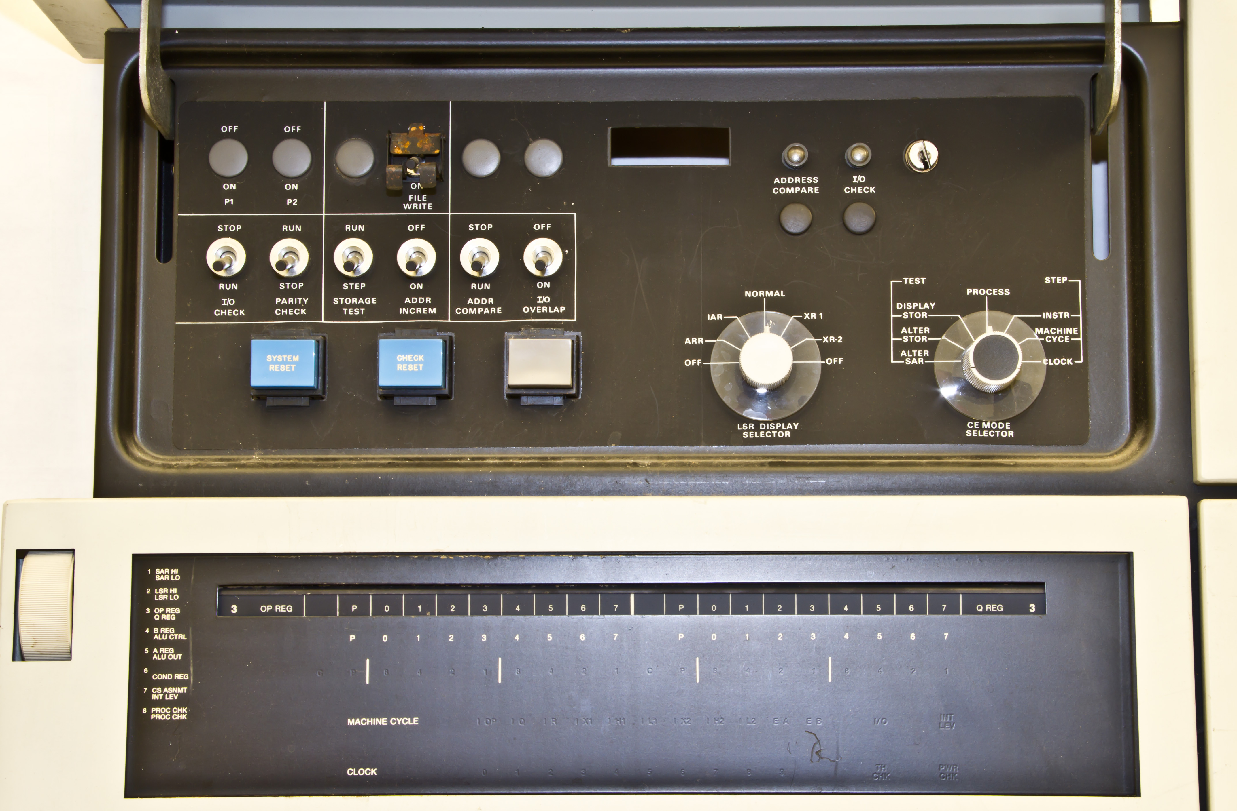
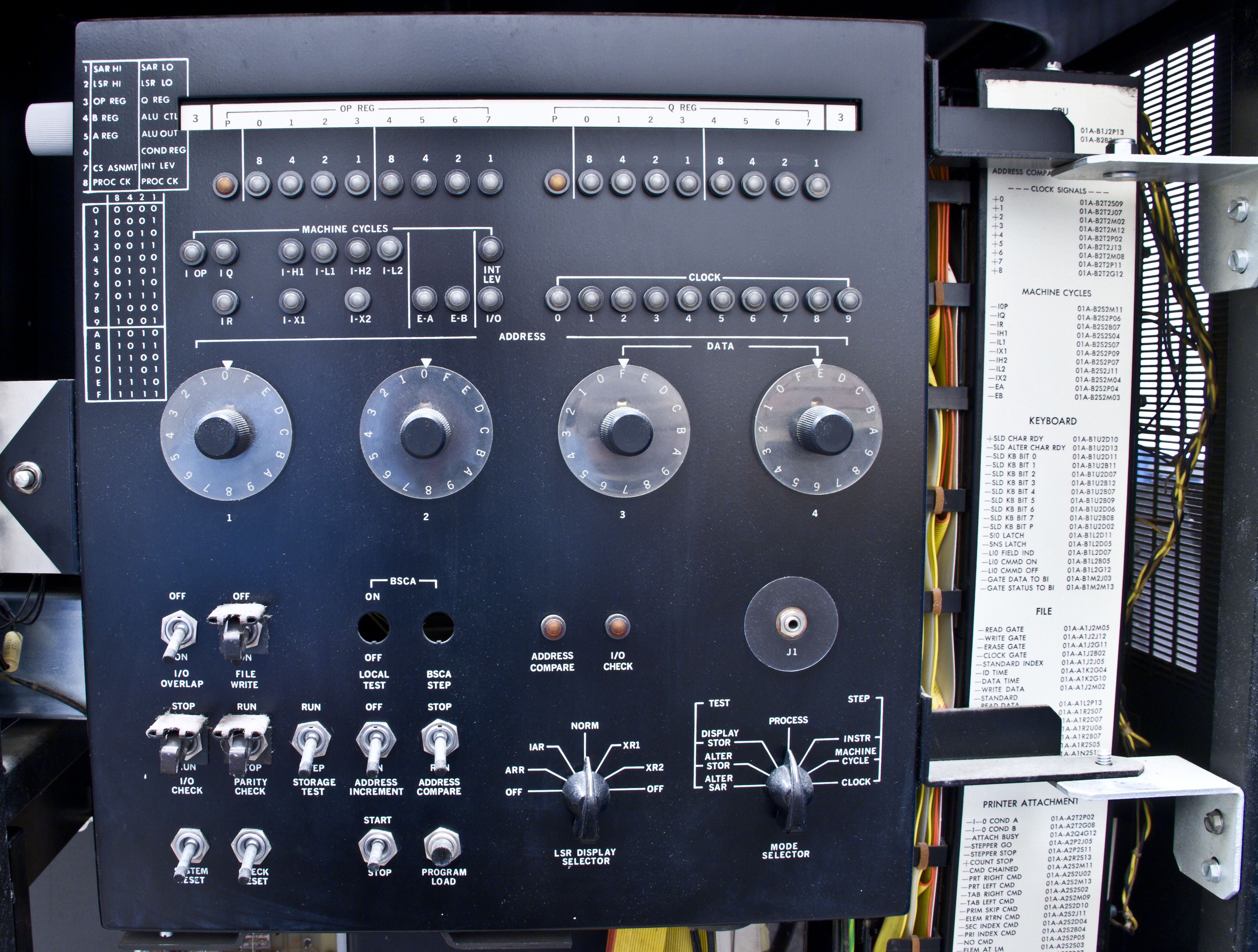
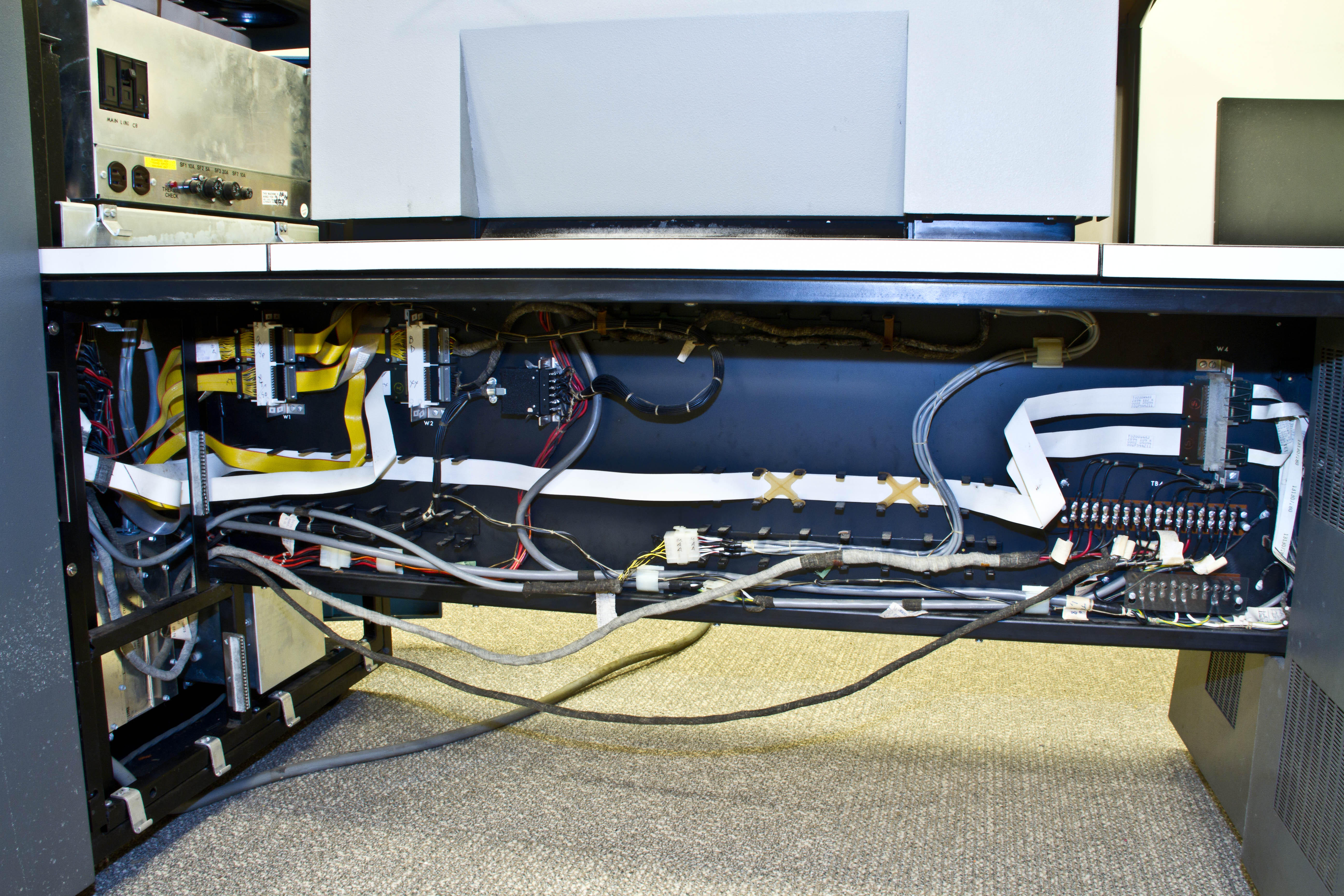
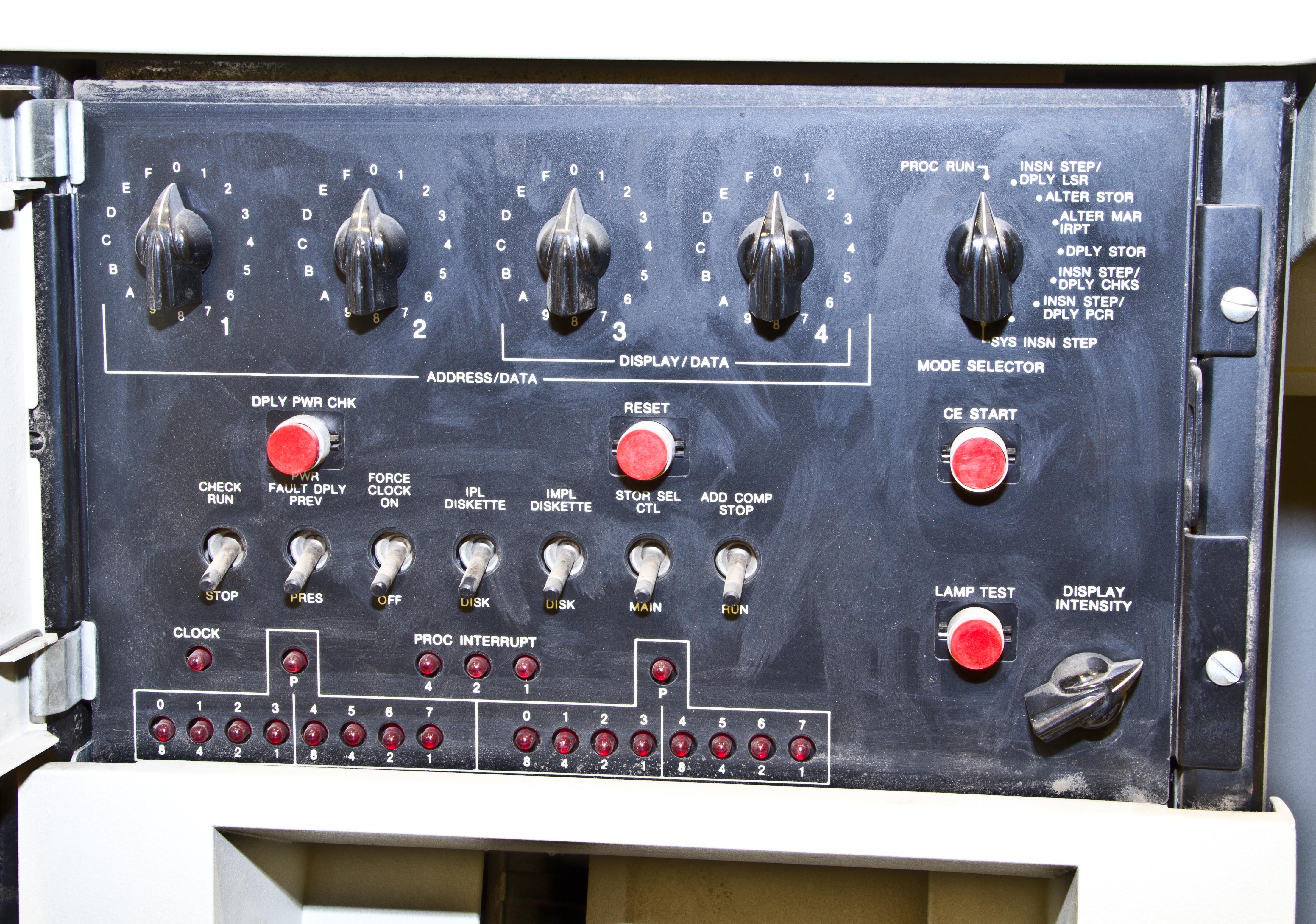
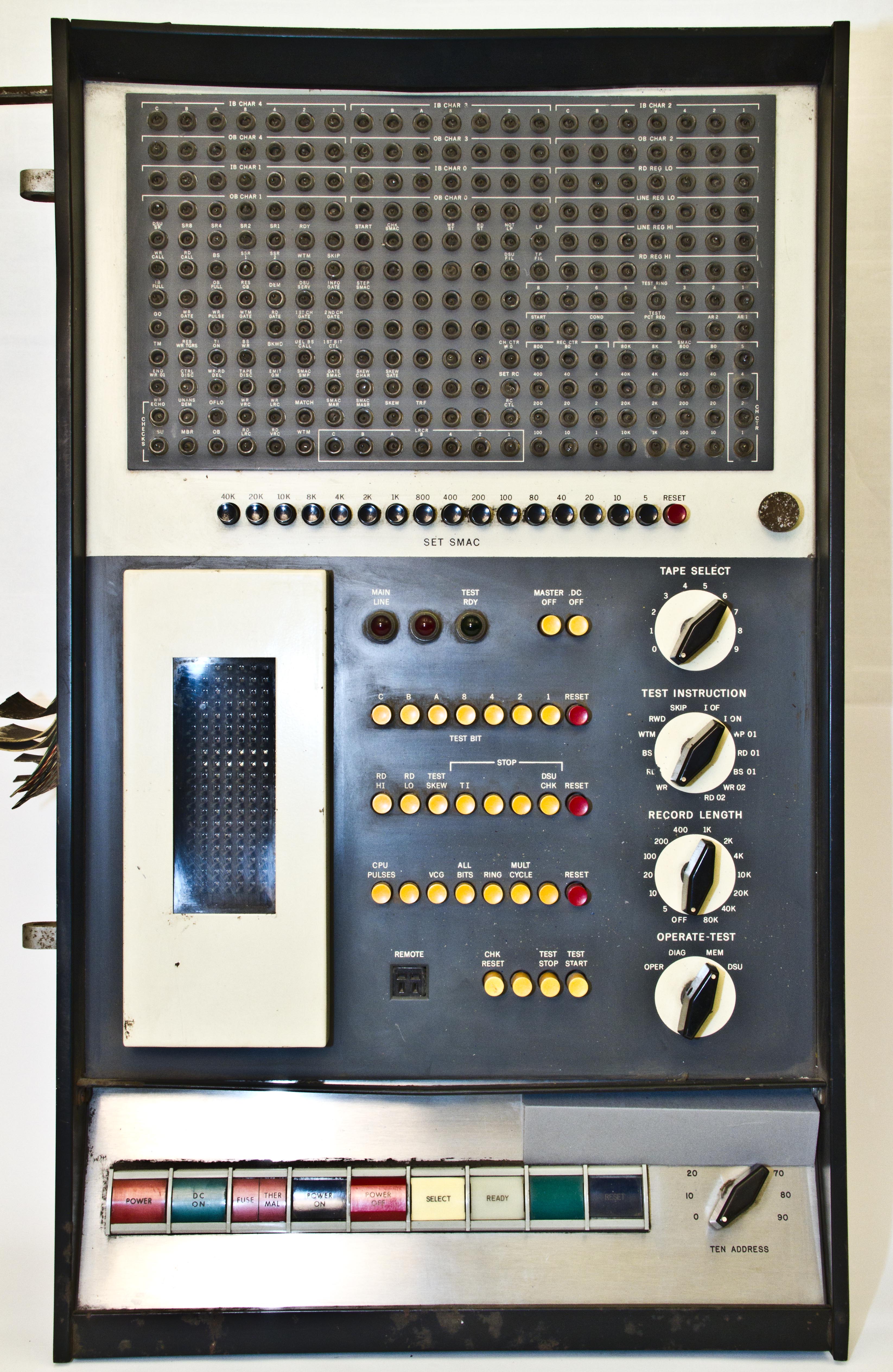
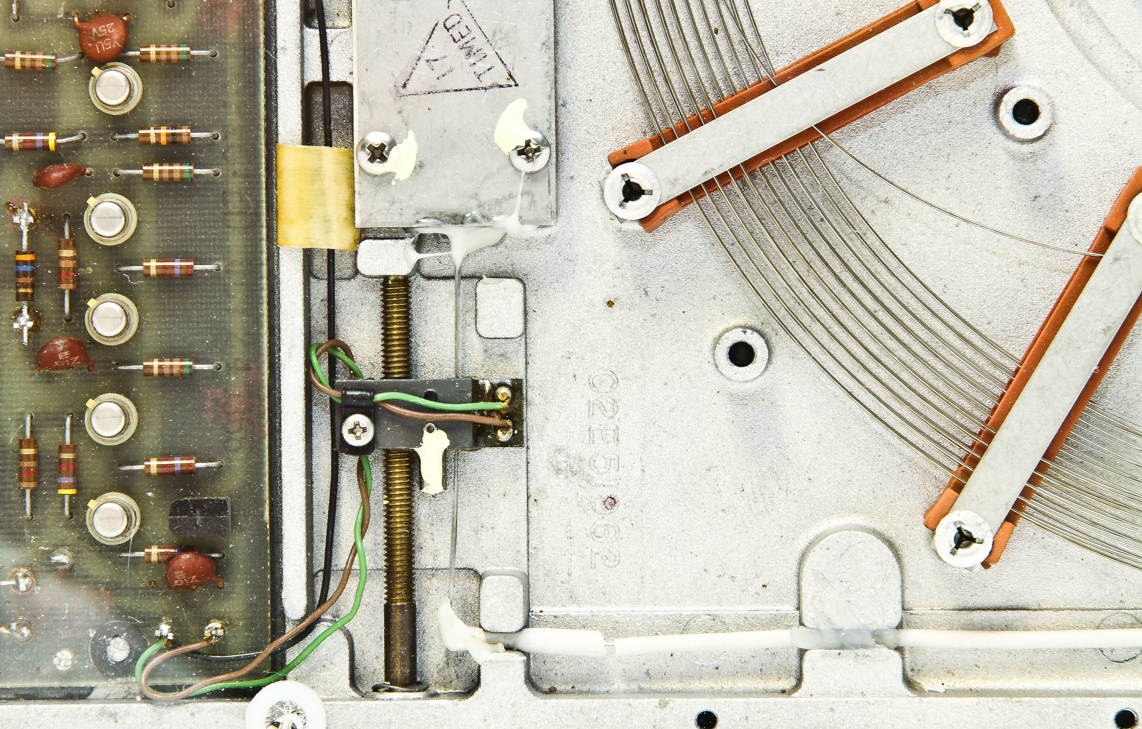
Figure 12 shows the CE (Customer Engineer) control panel. This was our primary debug tool when I was developing code for this system. We would single step the code examining processor state using the lights. You could also easily modify memory from this console. Figures 13 and 14 show the back view of the system including the cables the connect the two halves together. For shipping and installation, the system could be separated into two components: the "table" part, and the "box" part. (Our system had to be separated into two pieces in order to get it though doors.)
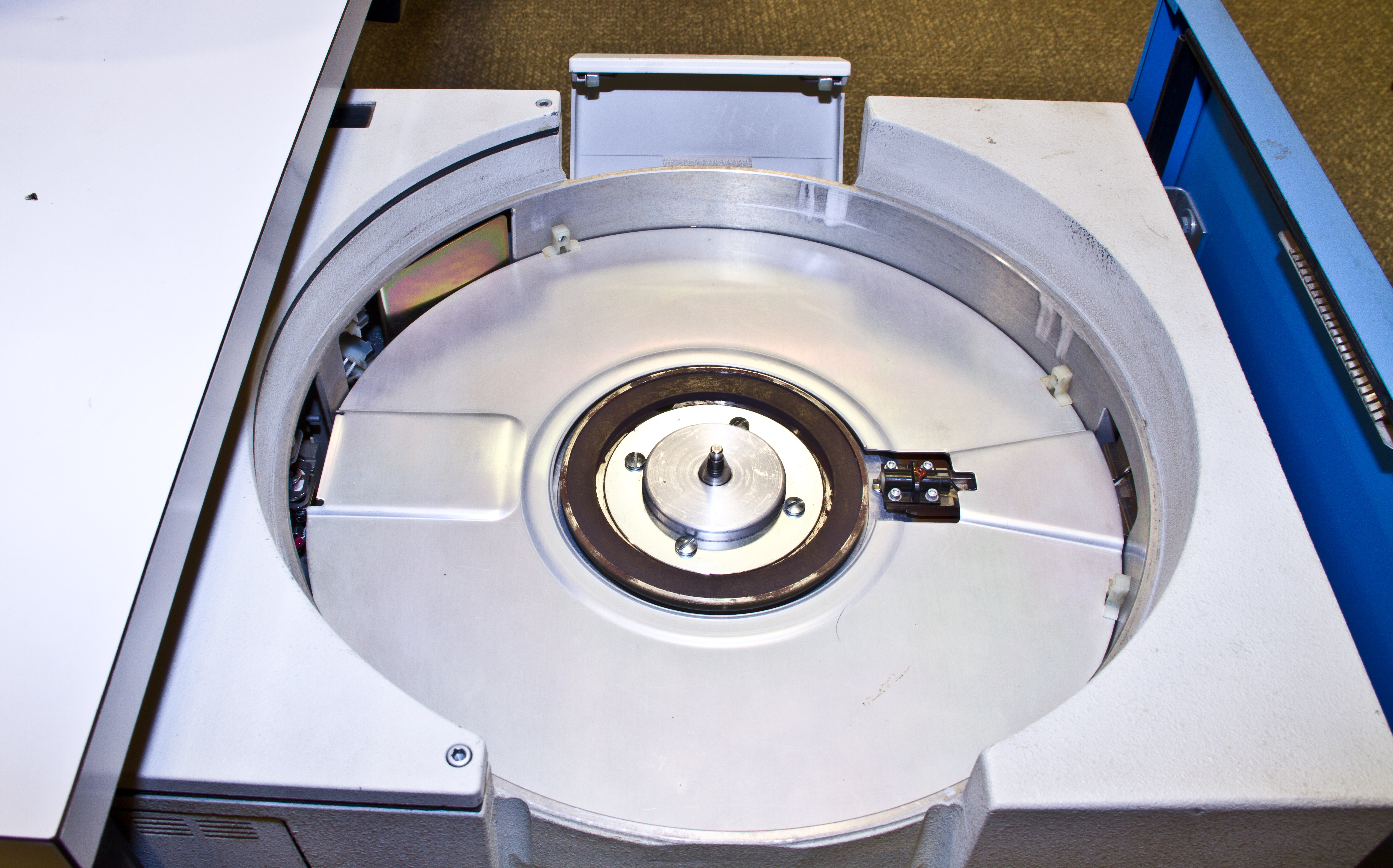
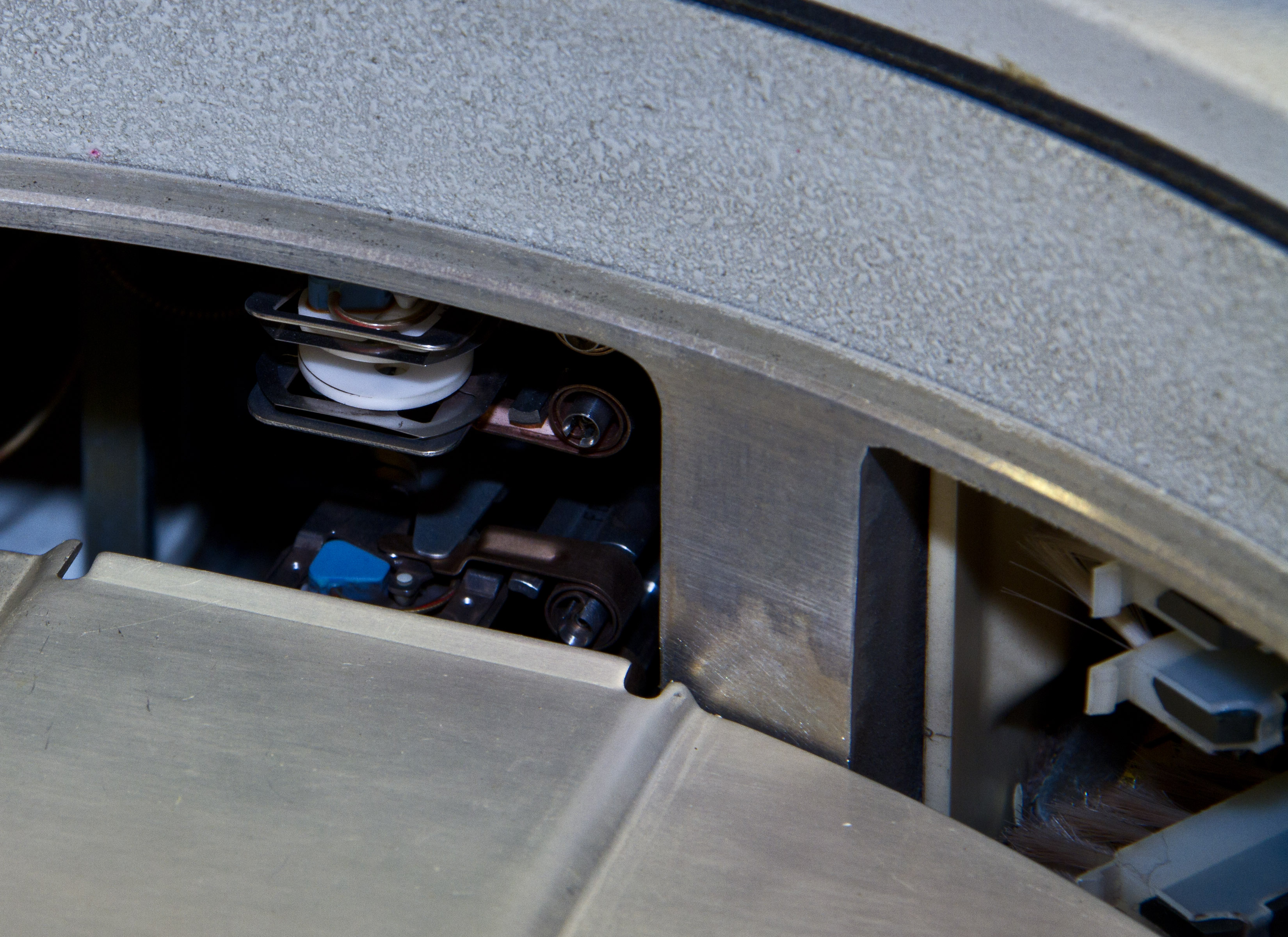
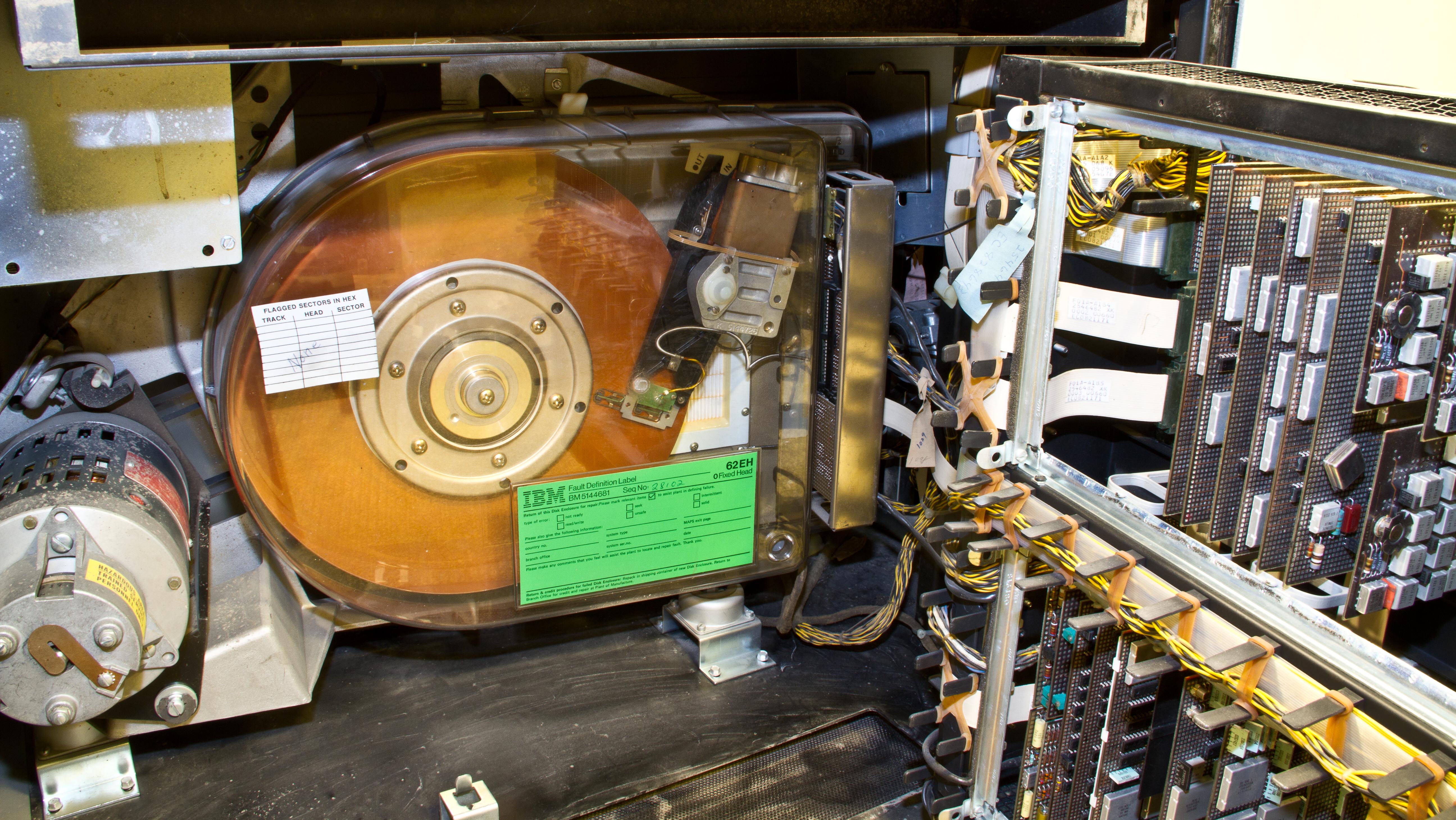
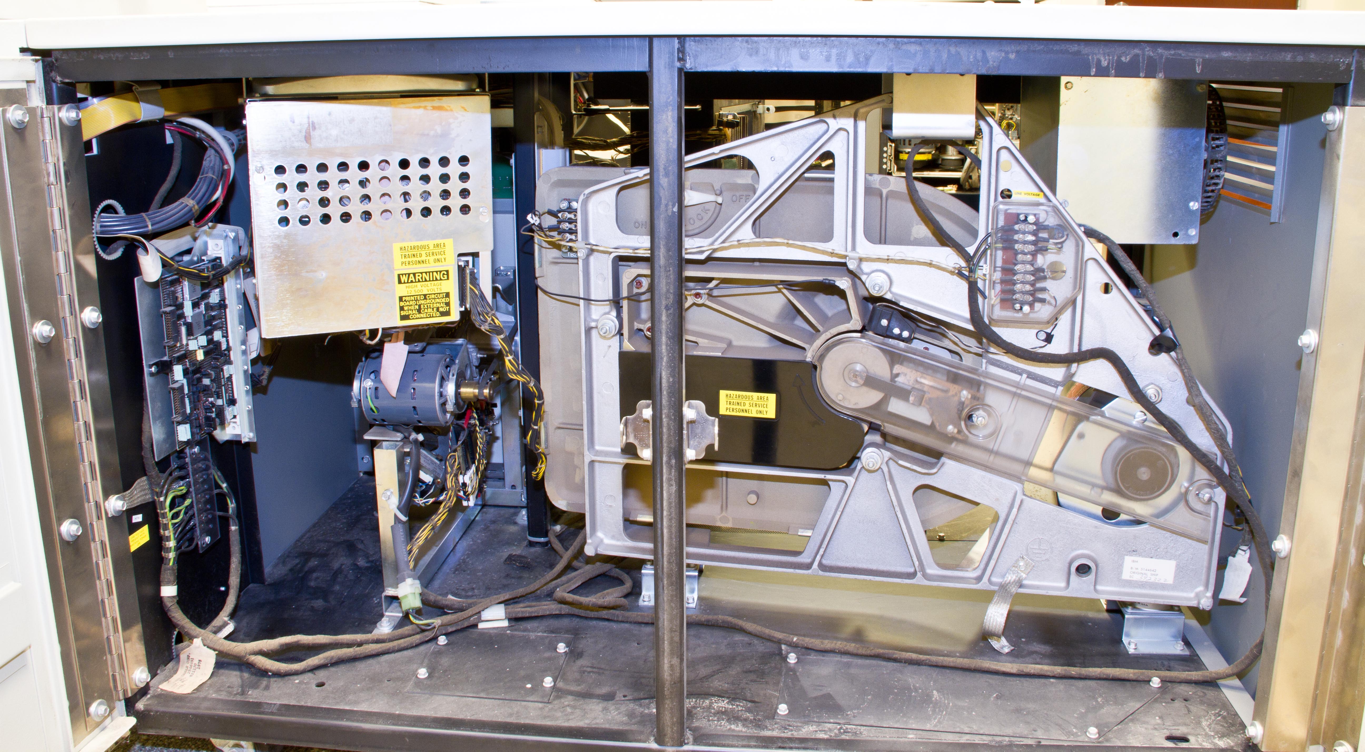
Figure 15 shows the back of the 5444 disk drive unit at the left of the table (from the front). There is a compartment for a second 5444 under this, but our system only has one disk drive. There were two models of this drive; the larger had a capacity of 5MB split equally between a fixed platter and a removable platter.
Figure 16 shows the disk drawer opened with the removable disk installed. Below this is a fixed disk platter that shares the same access arm as the removable disk. Figure 17 shows the disk drawer with the removable disk removed. The fixed disk is barely visible through a hole on the right (where the index transducers are). Figure 18 shows a view looking at the retracted heads and the cleaning brushes on the right.
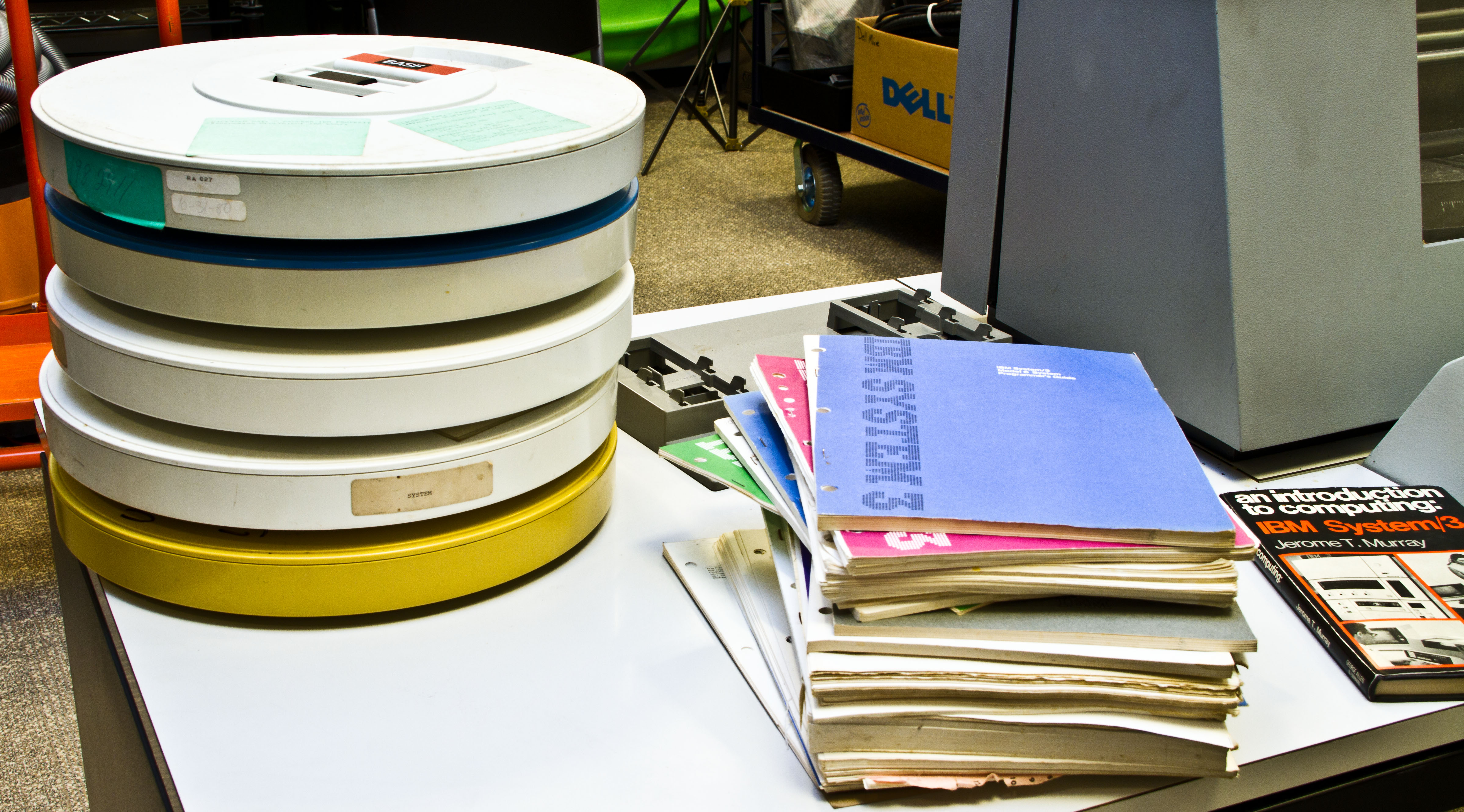
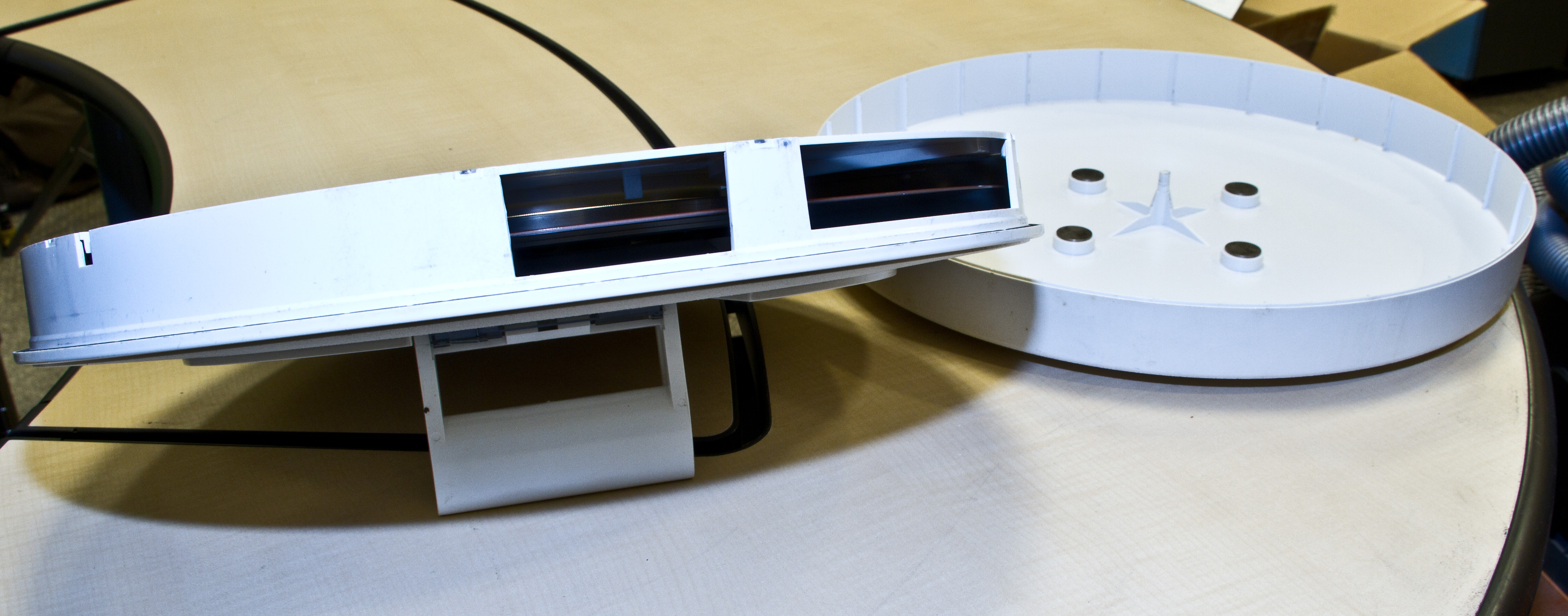
Figure 19 shows some of the documentation received and five disk cartridges containing system software. Figure 20 shows 12 more cartridges that we have. Figure 21 show a closeup of the removable disk cartridge with the access holes for the heads and cleaning brishes.
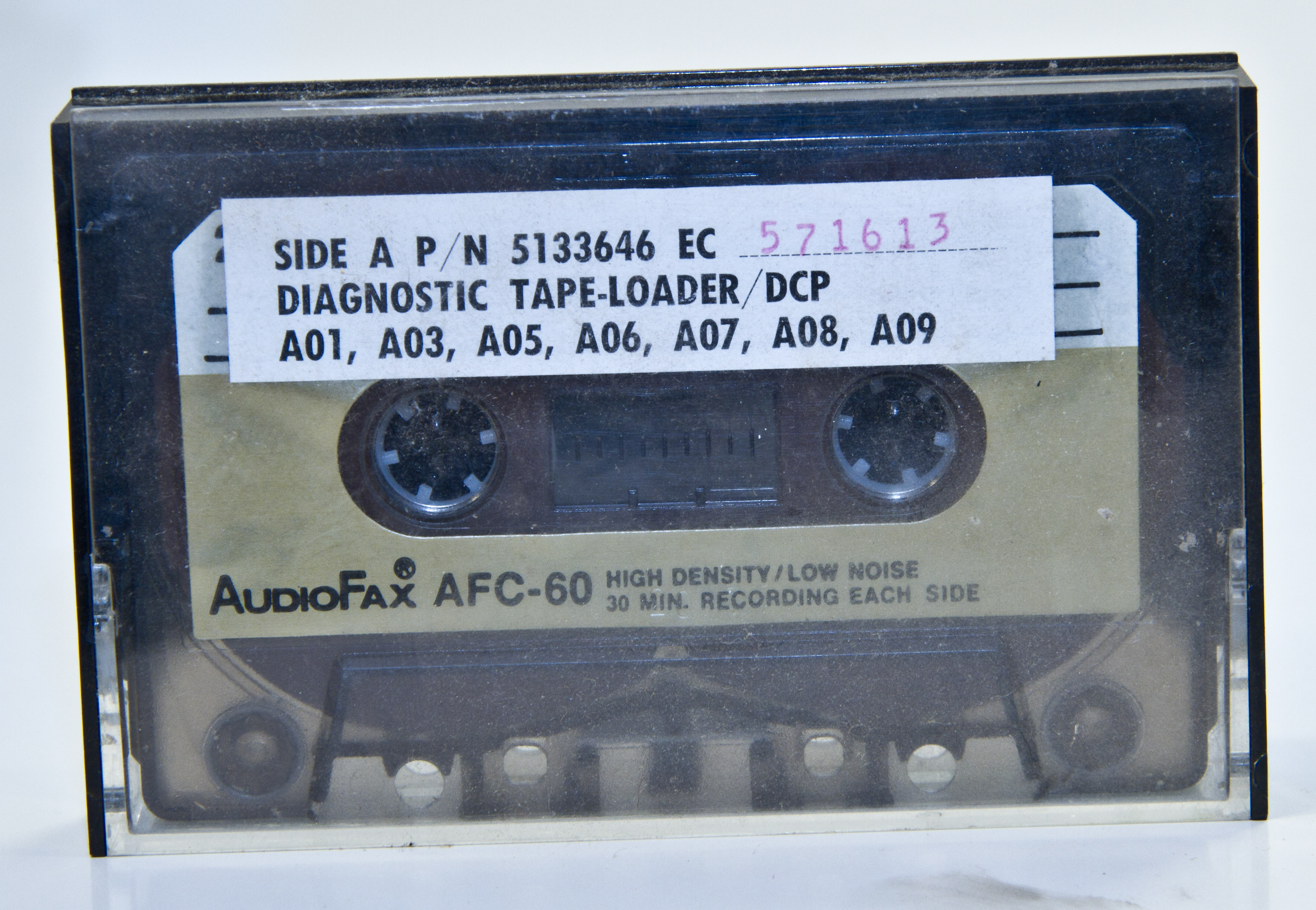
Finally, Figure 22 shows the a cassette tape used by the IBM Customer Engineer to run diagnostics and deliver software fixes. This was used since the only removable medium is the disk cartridge, too large for the CE to haul around. So, looking at Figure 12, there is an audio jack ("J1") used to plug in a ordinary tape player.
Announced in early 1975, the IBM System/32 was the lowest cost IBM offering (at the time) and became very popular.
It was a small single-user business-oriented computer that was less expensive than the System/3 Model 6 (some models leased for less than $1,000 per month. The System/32 was designed for business applications (e.g., billing, inventory control, accounts receivable, sales analysis, etc.) written in RPG.
The system was a single desk-sized unit comprising a processor, fixed-disk storage, a data diskette, a printer, and an operator console with a small visual display screen. The System'32's tiny display contained six lines of 40 characters each. Solid-state main storage was available in sizes from 16K to 32K bytes. A emovable contained around 262 KB, and the fixed disk options were approximately 5 or 9MB. Two communication options were available (BSCA and SDLC) supporting data rates up to 7200 bps.
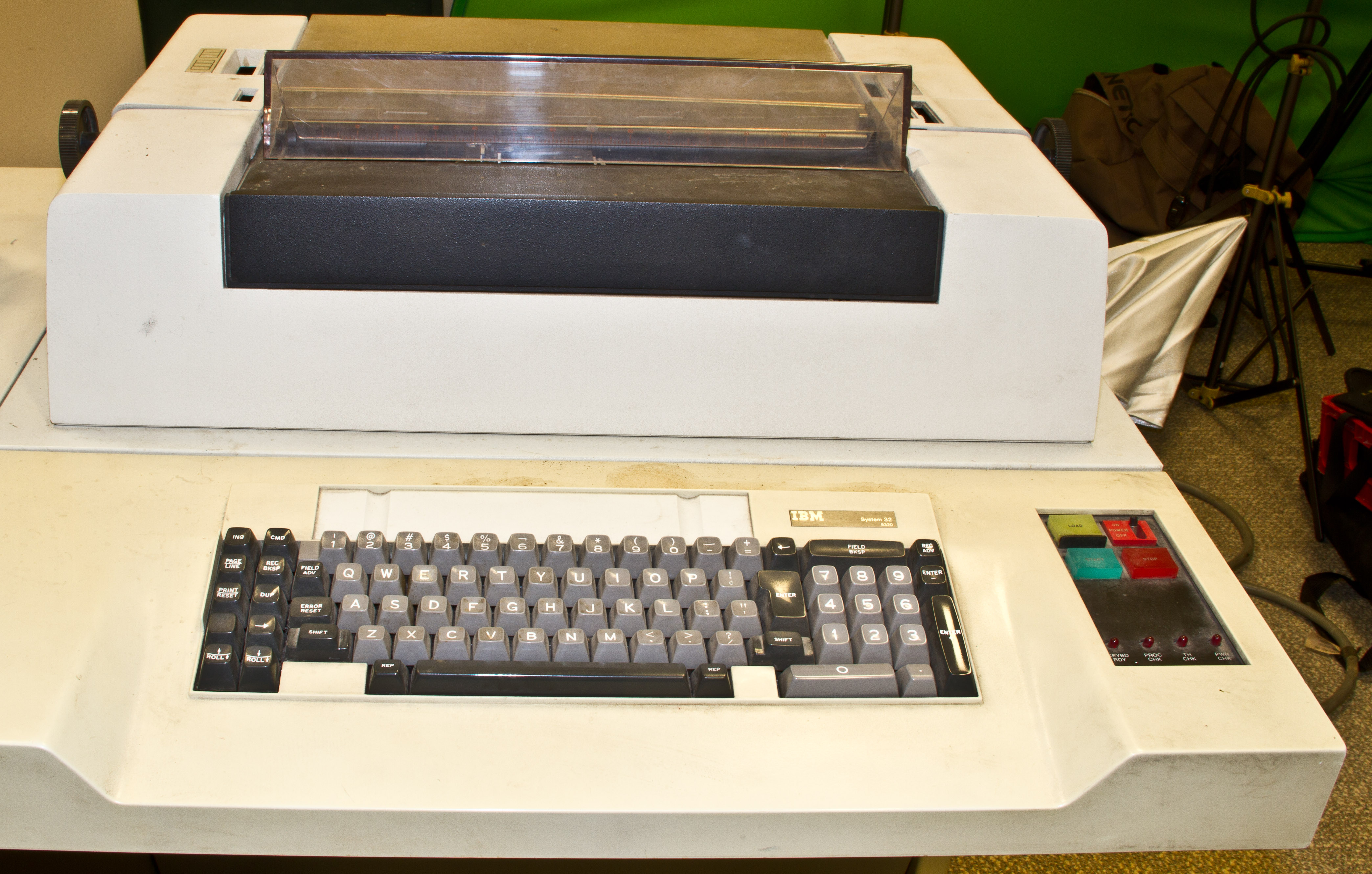
Figure 1 shows the complete System/32 (the weird photo angle is to mask a huge amount of junk in the room). Figure 2 shows the operator station with the small display on the left and the printer behind the keyboard, which is shown in more detail in Figure 3. Figure 5 shows the hidden CE panel (in front of which I spent many nights, see below). Swinging the logic gate out, we see in Figure 5 the giant disk drive. Figure 6 and 7 show the front and back of the logic gate. This small amount is the entire logic in the system (other than the CRT control logic and without the optional communications feature). Figure 8 shows the back of the unit with the vertically mounted CRT in a shield to the left of the disk drive. The motor for the diskette reader is alos seen below the CRT shield.
From an application viewpoint, the System/32 had the same instruction set as the System/3 models and the system software (SCP) was very similar to that of the System/3 Model 6's. Similarly, the primary application language was RPG. Due to its small business orientation and low cost, the System/32 was very successful: according to the IBM link, it became the most installed IBM computer of the 1970's.
Even though the System/32 appeared to software to have the System/3 instruction set, internally the processor did not directly execute System/3 instructions. To minimize cost, the I/O devices were very "dumb" and the processor (called the Control Storage Processor, or CSP) was optimized for low-level control of the I/O devices. The code executing in the CSP (called microcode) was contained in a writable control storage and included an emulator of the System/3 instruction architecture.
Microcode for the System/32 was much simpler than the typical "horizontal" microcode as implemented on other IBM processors. The System/32 processor had what we would later call a RISC architecture. Instructions were 16-bits wide and addresses were 16-bits wide. The microcode control storage was 4K 16-bit words (an extension of another 4K was available and contained emulation of floating-point arithmetic). Four usable interrupt levels each had eight 16-bit general purpose registers. All logical and arithmetic instructions were register-to-register operations. Main memory was accessed only by load and store instructions. There were condition flags for branching and only about 19 basic instructions. Of course, there was no pipelining, no caches, no branch prediction, or other performance features like are common on modern processors.
A CSP instruction executed in, on average, five to seven 200ns clock pulses. That is, a CSP microcode instruction instruction executed in about the same time as the 1.5us processing of a byte in the memory-to-memory architecture of the System/3. Since emulation of a System/3 architecture instruction tool many microcode cycles, emulation of System/3 was very slow. This lead to the innovation of moving some of the SCP into microcode (discussed more below).
In 1970, I finished my work on system software for the IBM System/3 Model 6. I then worked on the architecture of another proposed small computer, which was killed and the key personnel asked to move to Rochester MN. I was offered the job of the second line manager developing the operating system (the System Control Program, in IBM terminology) for a new small computer system (which ultimately became the System/32). So, in 9/71, I moved to Rochester (getting married to an IBM programmer on the way).
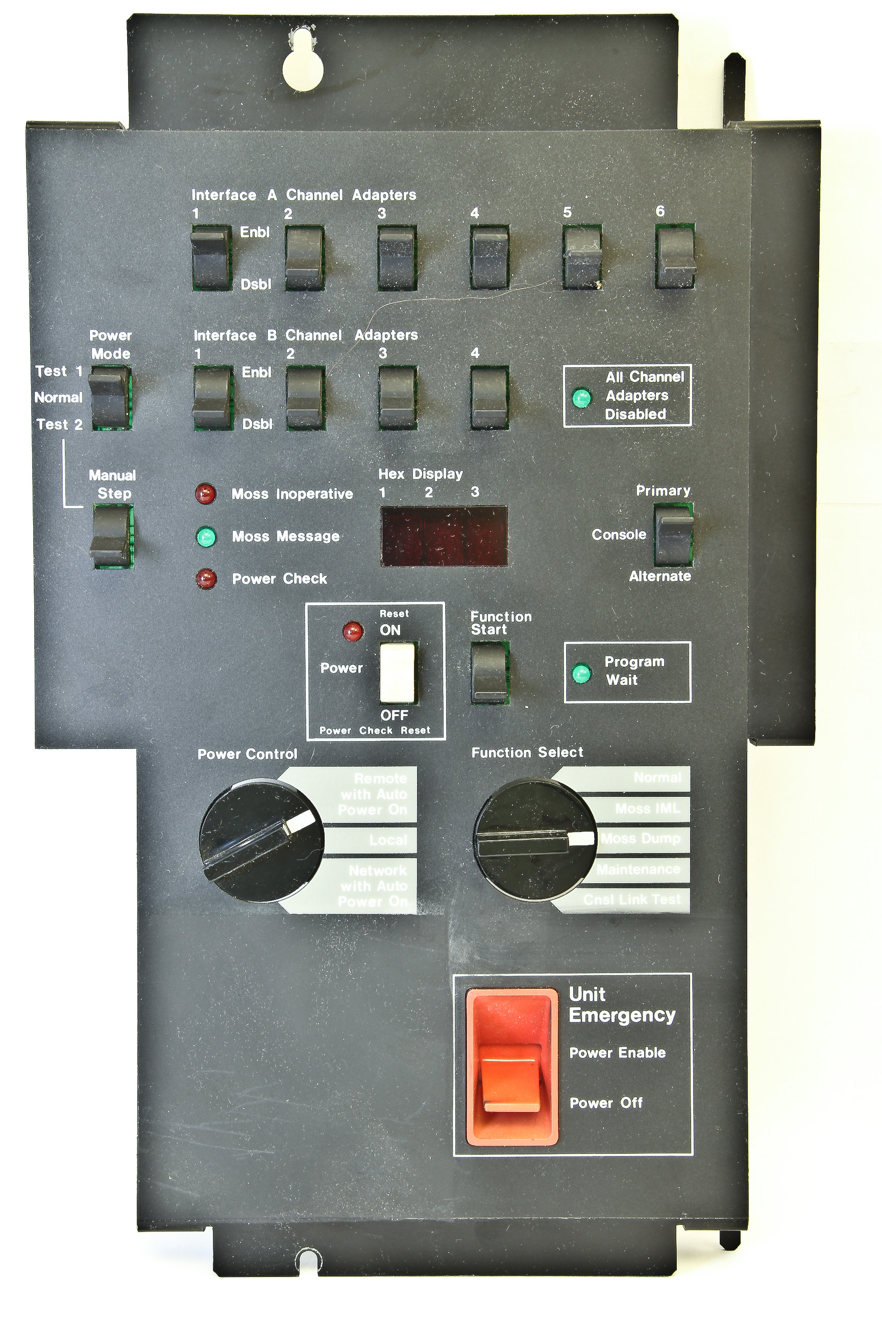
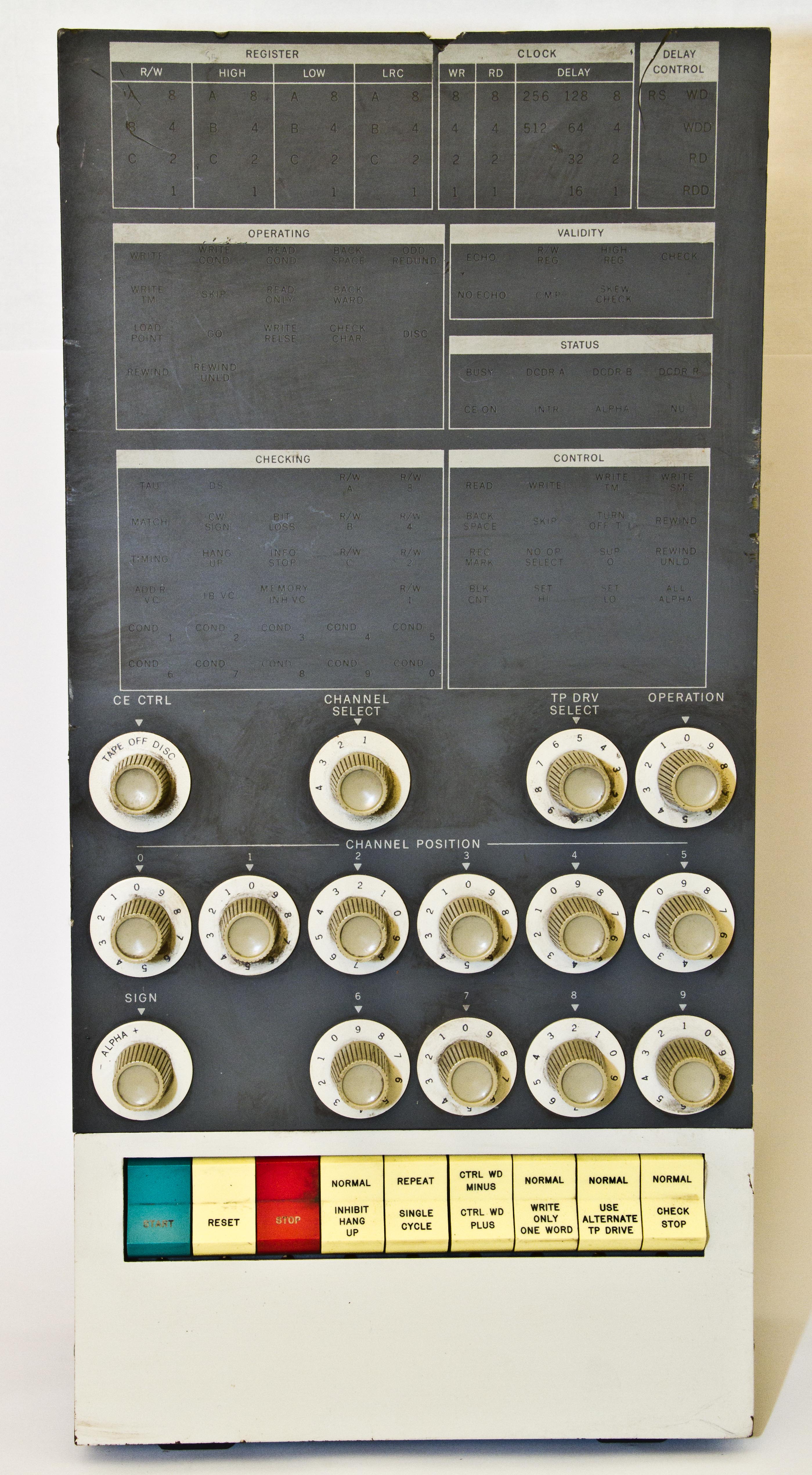
As well as being the manager of the system software development, I proposed and personally coded microcode that implemented some of the disk management functions of the operating system in microcode. While this seems obvious now, at the time I believe this was the first time this was done in IBM (moving SCP functions into microcode). I vividly remember watching the 1972 Olympics at home nights while also translating the System/3 SCP disk management code in microcode. There was no simulator of the CSP; the only way to debug code was on the hardware. Machine time was hard to get since there were few models available and the engineers were busy working on them. Thus, I mainly found time to use the hardware at night. I remember long nights sitting in front of a very early hardware model and debugging my code using the control panel shown in Figure 4 (the only debug mechanism available). Due to the developing nature of the hardware, I also found a few bugs in the hardware.
The museum acquired the System/32 from its original owner in a small ranching and farming town in Oregon. This information came from its only owner before the museum acquired it:
"I bought it new in the 70's for a farm machinery business to do bookkeeping and some inventory control. There were no bookkeeping software packages tailored for the 32 at that time, so the IBM sales folks found me a system 3 package and a programmer to modify it to run on the 32. My training to this point was a degree in engineering using a slide rule. I worked with the programmer and the wonderful instruction manuals and learned RPGII and went on to write many programs for the 32 and my business."


Extensive microcode allowed the System/360 to provide a compatible instruction architecture and compatible I/O across many models having significantly different performance. Among the original offerings, the Model 30, 40 and 50 all had hardware significantly less powerful than the System/360 instruction architecture and implemented the instructions via microcode.
The microcode was contained in a control store implemented as read-only storage, or ROS (this is IBM's term, today we call it read-only memory, or ROM). Then, as today, ROS is implemented as a two-dimensional array of word-lines, which select the output for a particular address, and the orthogonal bit lines which are the outputs. Since only one word line is active at a time, the output for each bit of selected the ROS word can be defined by either no connection at the intersection of the word-line and bit-line, or by connecting the word line to the bit line through a diode. That is, when a bit-line is asserted, the output of the ROS is defined by the connects or no connects to the bit lines for that particular address. The difference among the many implementations of ROM are primarily in the choice of this connection mechanism. Different types of "diodes" affect the speed, size, and ability to change the ROS.
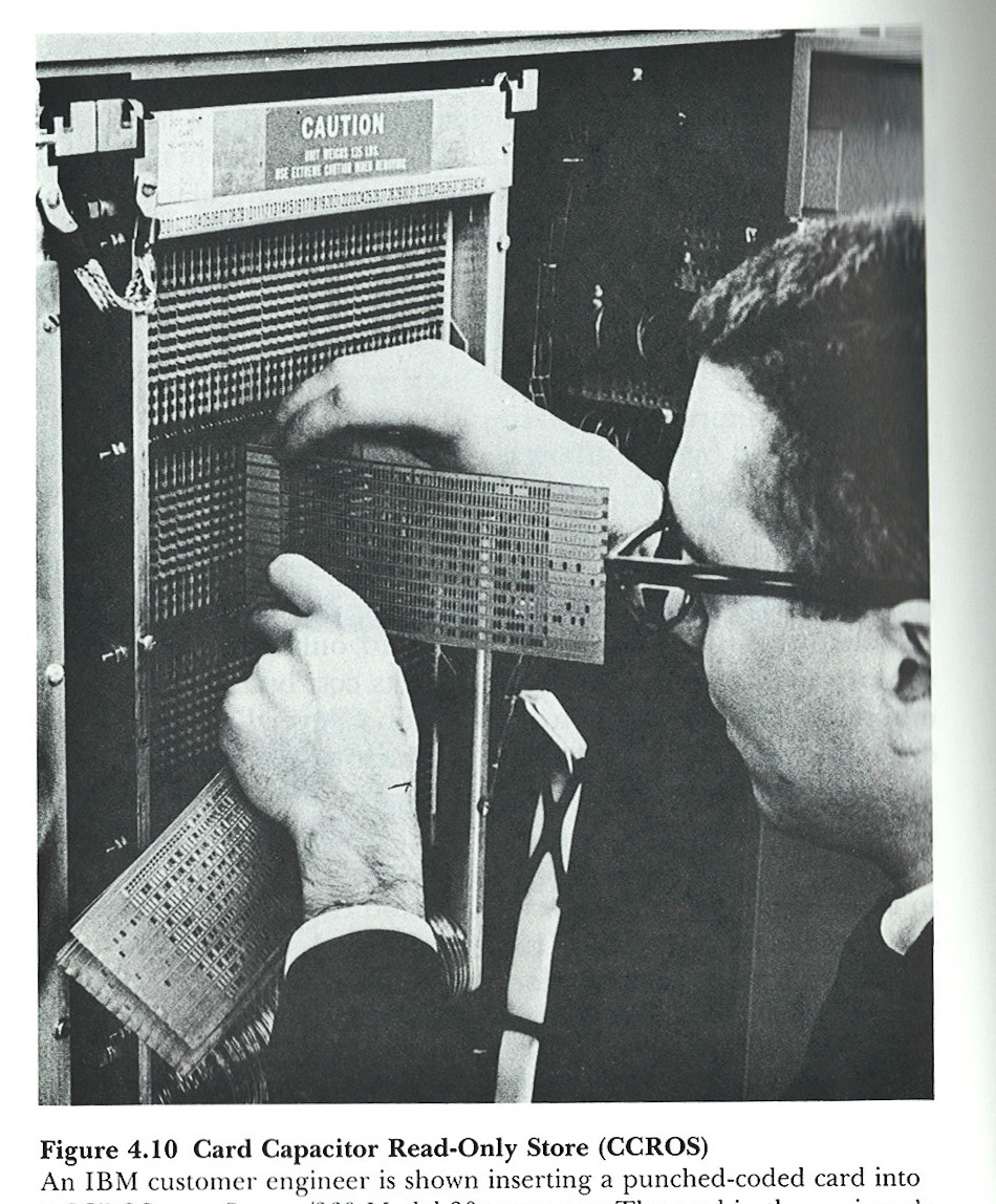
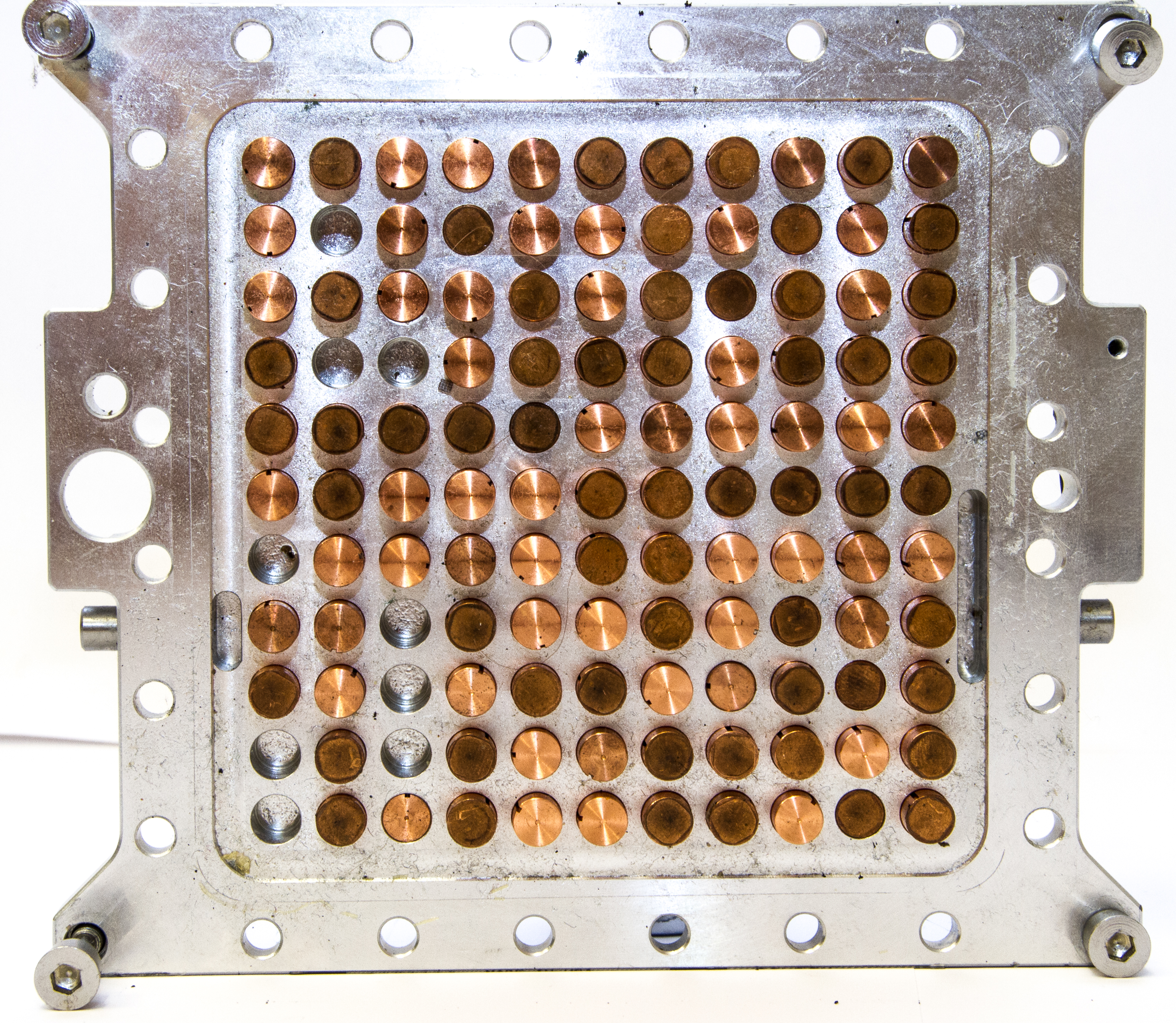
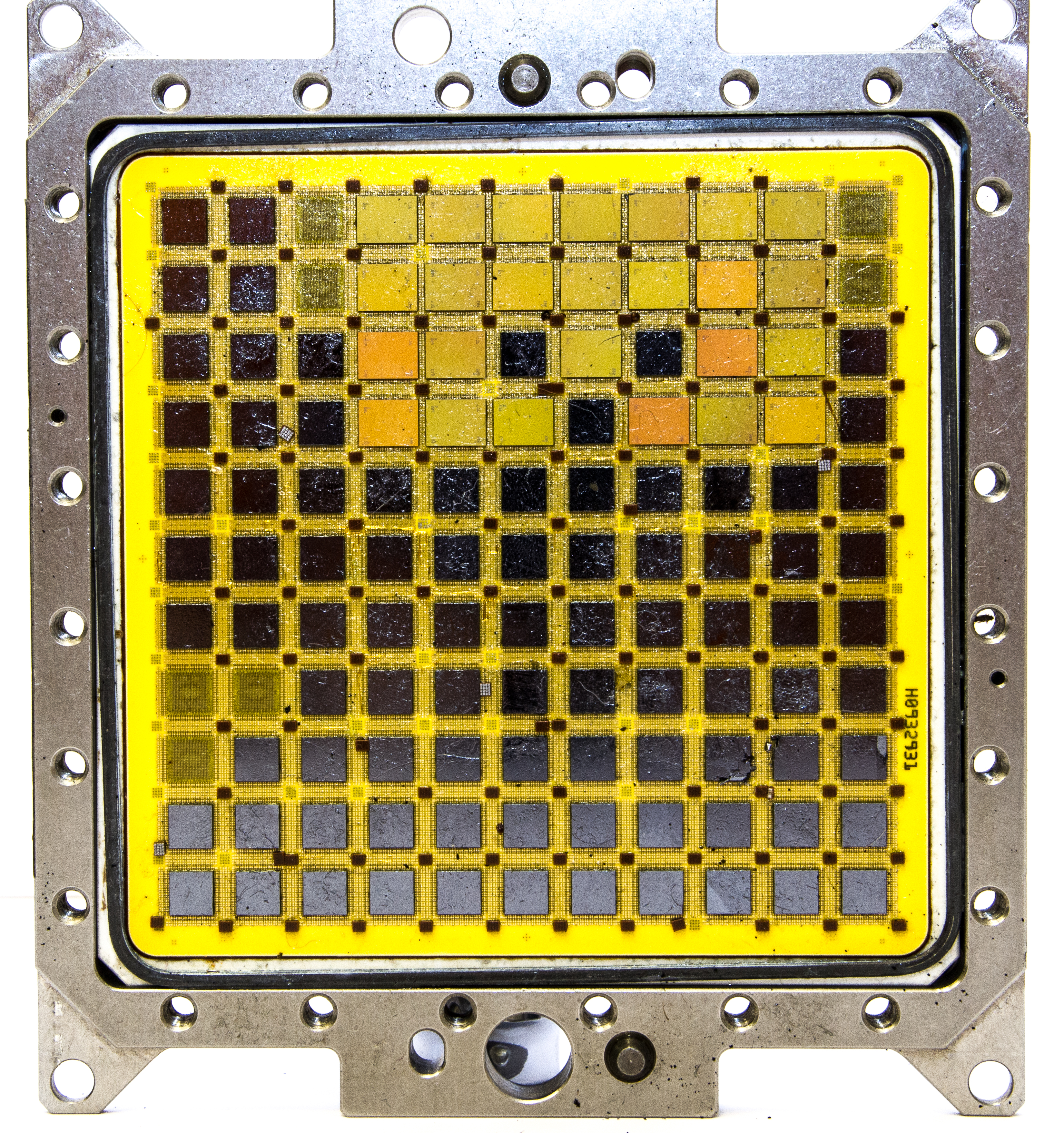
All except the high-end model of the original introduction used microcode to implement the System/360 architecture. Three different types of ROS were used: Card Capacitor ROS, Transformer ROS, Balanced Capacitor ROS. We have samples of all three of the types. Figure 1 shows a storage card of the Model 30's Card Capacitor ROS. The storage card looks like an IBM punched card except it is made of Mylar and has metal lines etched on it. (Much more about this ROS design can be found in J.W.Haskell,Design of a Printed Card Capacitor Read-Only Store, IBM Journal, March 1966.) Figure 2 is a closeup of the card.
Each card has 12 word lines corresponding to the 12 rows on a standard punched card. The contacts for the word lines are on the right in the picture. Each word line attaches to 60 bit "pads" (again corresponding directly to the punch positions in a standard IBM card). The metal pad can be eliminated by punching that position with a standard card punch. Thus, bits in the microcode word for each word line are defined by the metal pad being present or absent.
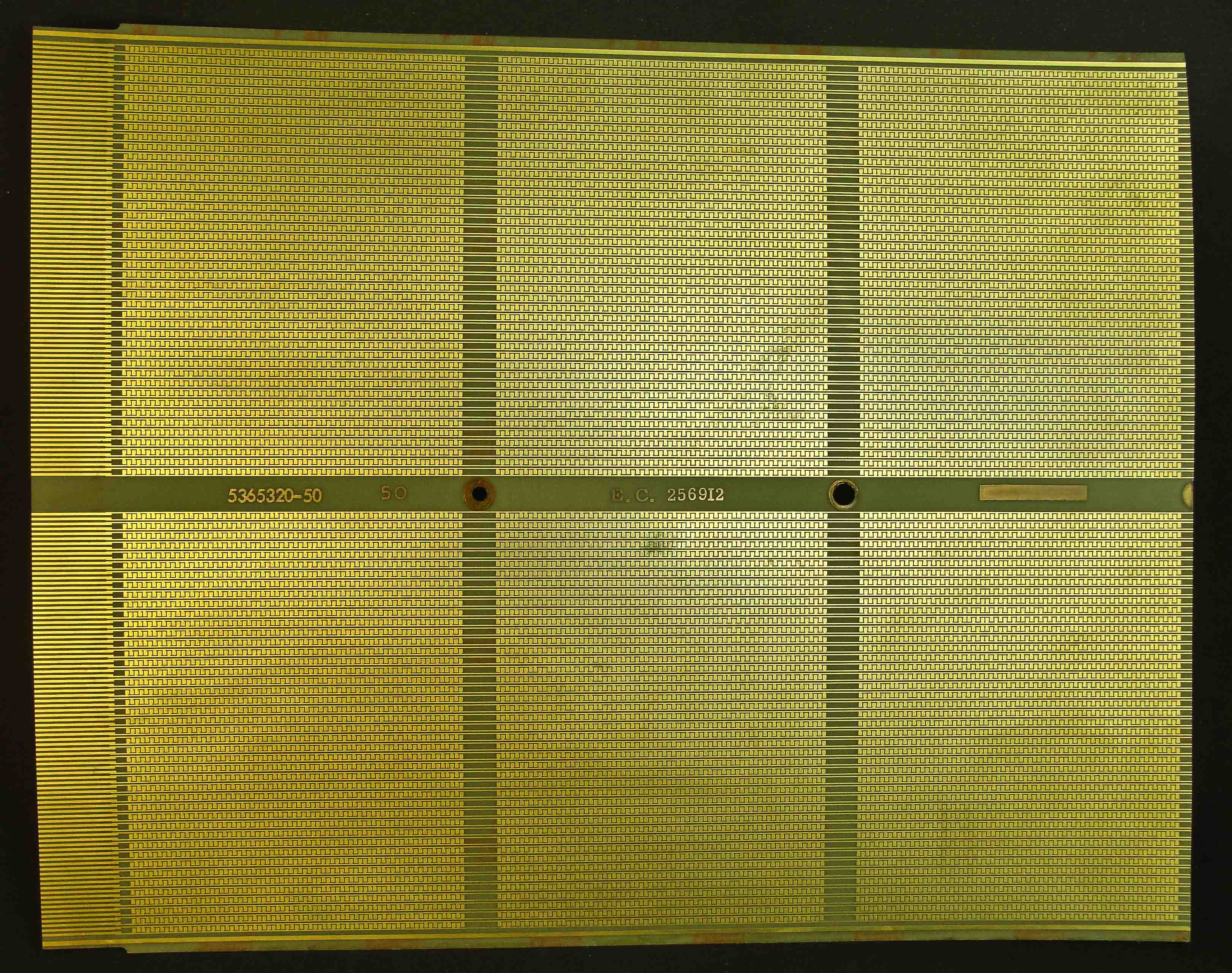
The ROS cards are placed in a frame where bit lines run vertically aligned with each of the 60 column. A thin sheet of Mylar goes between the card and the bit lines to form the capacitive coupling between the metal pad and the word line. The cards are mounted on a 20x12" board with four cards on each side. The mechanics of the boards (ground planes, pressure on the card, insulator thickness, etc.) are such that the coupling ratio between a punched and unpunched pad is at least 10:1. The boards are assembled into a module to form the complete ROS. The Model 30 ROS used 43 boards for a capacity of 4032 60-bit words (with one spare board). The access time for this ROS is 0.75 microsecond.
It was relatively easy to change ROS cards in installed systems. This flexibility was important because the Model 30 had an option to emulate the machine instruction set of the very popular IBM 1401. Figure 9 (taken from another source) show IBM Field Engineer changing the ROS for a Model 30.
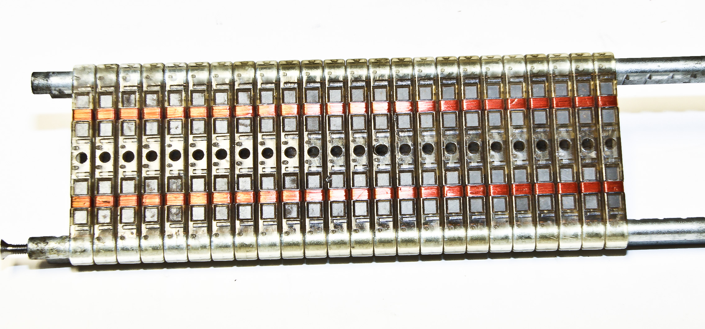
Figure 3 show the code portion of a module from the Model 40 Transformer ROS. Instead of a capacitor forming the connection between the word line and the bit line, the TROS used a transformer at the intersection. Figure 4 is a closeup of one of the Mylar strips containing two 54-bit ROS words. The word line is etched on the strip and completes a loop from one end back to the same end. The current is routed in one of two ways around a central metal core for each bit. The current direction around the core determines whether it is sensed as a 0 or 1. The current direction is controlled by punches that disconnect one side of the current loop around each bit post. (Much more about this ROS design can be found in D.M.Taub,T he Design of Transformer (Diamond Ring) Read-Only Stores, IBM Journal, September 1964.)
Figures 5 & 6 show the "bit line" sensing mechanism that sits on top of the metal cores for each bit. Each module has 128 tapes, each storing 2 words. A total of 16 modules formed the ROS for the Model 40, for a total of 4K words. The access time was 240ns with a cycle time of 625ns. Figure 8 shows 8 modules of the Model 40 ROS; another 8 modules are behind the visible ones.
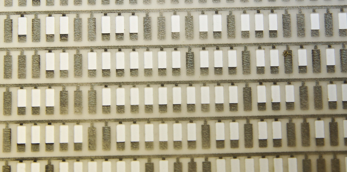
Figure 10 is part of the Balanced Capacitor ROS of the IBM System/360 Model 50. It is called balanced because the capacitance load on the word line is the same regardless of the pattern of bits. This is as opposed to the Card Capacitor ROS shown in Figure 1 where the number of 1 bits changes the word line capacitance. The balanced approach allows a faster access time: the timing of the Model 50 was 90 ns access and 200 ns cycle. The disadvantage of the balanced approach is that the bit patterns have to be manufactured into the card, as opposed to the card capacitor approach where new ROS bits can be created on site.
Figure 11 shows a closeup of the card. A ROS bit is represented by two locations along the word lines. There are two "word" line for each bit: one is the drive line to trigger reading. Attached to this line is one "pad" shaped per bit. There are two sense lines for each bit on the sensing plane that the ROS cards are pressed against: one for 1 and one for 0. The position of this bit pad over the two sense lines determines whether it is represents a 1 or 0. The other word line a "balance" line for attaching the complement of the bit flags. For example, compare the first two bits of the top two bit rows in Figure 11. The first two bit pads are the same: the right pad is attached to the drive line. The next bits are different: top row has left pad attached, and bext row has right pad attached.
(Much more about this particular ROS design can be found in S.A.Abbas, A Balanced capacitor Read-Only Storage, IBM Journal, July 1968.)


The museum has a control console from a IBM 705 computer. I believe this to be very rare item since the 705 was first shipped in late 1954 and was withdrawn in early 1960. That's a long time ago and there can't have been many shipped during that short period (but I haven't found credible numbers for the total shipped). Also, the 705 was quite expensive: about $590,000 in 1954 dollars.
(Note that on our console the original IBM 705 banner has been replaced with a customer's banner ("Confederation Life"). Since computers were so rare in the 1950's they were usually proudly displayed in a "glass house" by their users, often with the user's name on them.)
The IBM 705 architecture was heavily optimized for business applications such as billing, payroll, accounts receivable, and inventory control, as opposed to computationally intensive applications. In early computers, hardware was so expensive and limited in capability that the each computer was specifically designed for certain types of applications, with a common differentiator being character handling vs. arithmetic computation. In the 1950's IBM introduced several 700-series computer starting with the pioneering IBM 701. The IBM 702, IBM 705 were optimized for business applications, while the IBM 704 and IBM 709 were optimized for engineering and scientific applications. Shown on the left is a pre-System/360 "family tree" drawing from IBM of its early computers which illustrates the various model and their introduction dates. This application optimization continued through later transistorized descendants of these 1950-era computers (such as the IBM 7080 which was the follow-on to the 705) until the introduction in 1964 of the IBM System/360 family, which had a "general purpose" architecture. Even after that, low-end IBM computers such as the IBM 1130, System/3, System/32, and System/38 were optimized for specific applications. And, process-control applications were addressed by the specialized IBM 1800, IBM System/7, and IBM Series/1 families.
The IBM 705 used vacuum tubes (about 1,700 of them) for its logic and used magnetic core memory for storage. Its instruction-set architecture was heavily optimized for business applications. Of special note is the fact that memory was organized into 7-bit "characters" and the two accumulators (corresponding to current processor registers) each contained 256 characters. The memory size was either 20,000 or 40,000 characters. A load from memory into the accumulator took about 17 microseconds. The main input and output was magnetic tape (5M characters per reel), but a card reader and punch as well as a printer could be directly attached.
In addition to the control console, we also have some electronic components and original documentaion (some probably rare) for the IBM 705. We have several of the pluggable processor logic elements as shown on both sides along with an ad for the IBM 701 showing the same type of pluggable unit. Also shown is our stack of more than 25 original IBM documents about the 705 including the introductory volume of the Customer Engineer (CE) internal documentation. This document describes the details of the logic elements and memory components.
New arrivals 12/2012
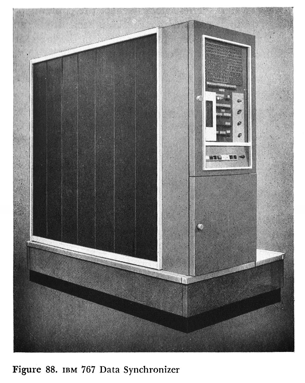
One of the most important peripheral I/O devices in a IBM 705 system was the IBM 767 Data Synchronizer. Figure 14 show a picture of the 767 from the IBM 705 Reference manual. The Data Synchronizer was the forerunner of what later became IBM's System/360 "Data Channels". It attached up to 10 IBM 729 tape Drives and allowed overlapping reads and writes across these devices to and from the main memory of the IBM 705. In today's terms it was a "multiplexed buffered DMA (Direct Memory Access) controller".
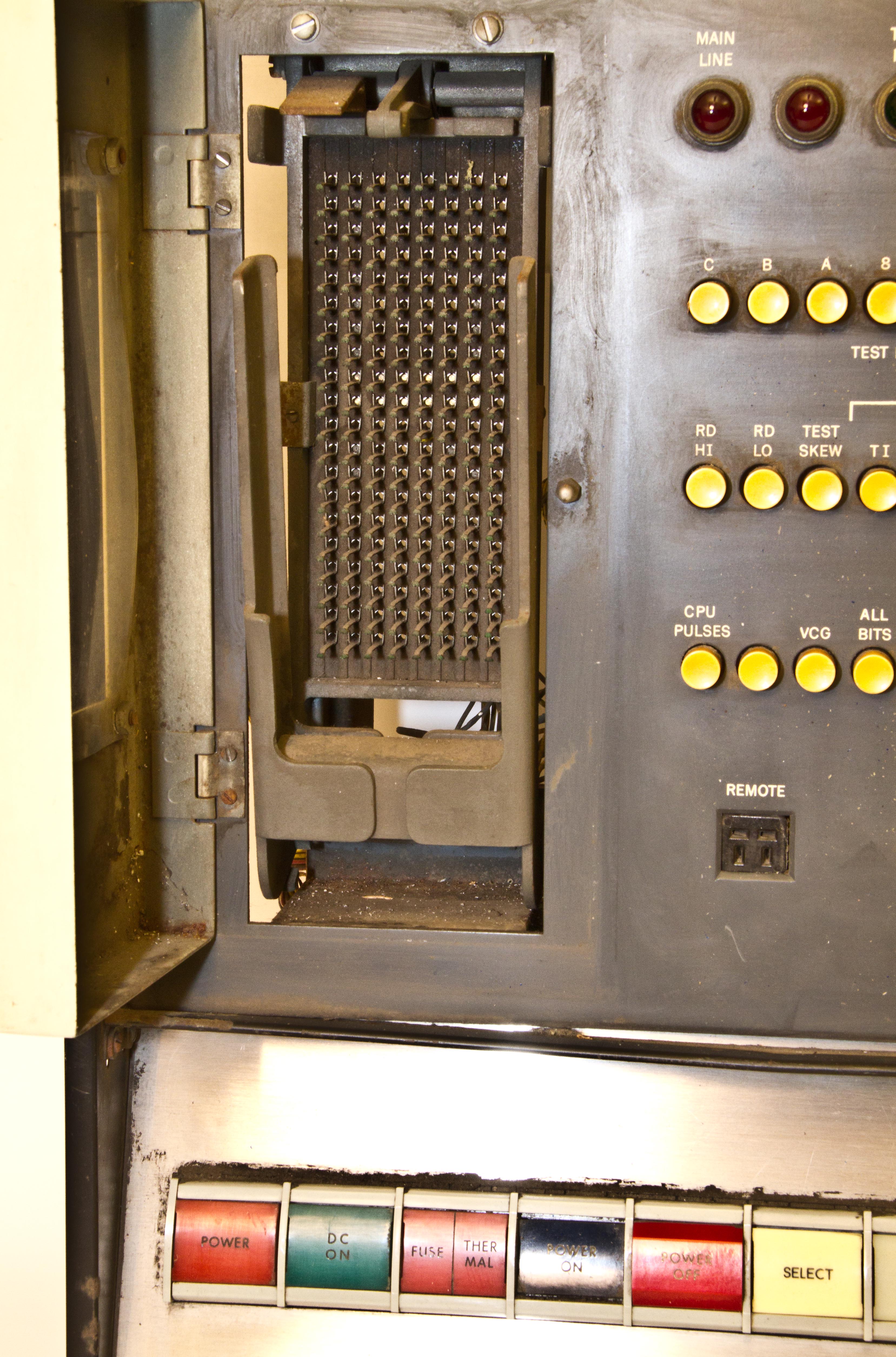
The museum contains a IBM 767 control panel, as shown in Figures 15, 16, and 17. Note that the front panel has a large bus connector on it.
Figures 18 through 21 show two other control panels that I am sure come from pre-System/360 IBM equipment, but I have not been able to identify them yet.


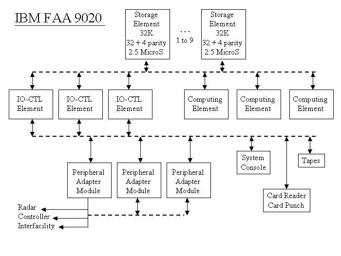
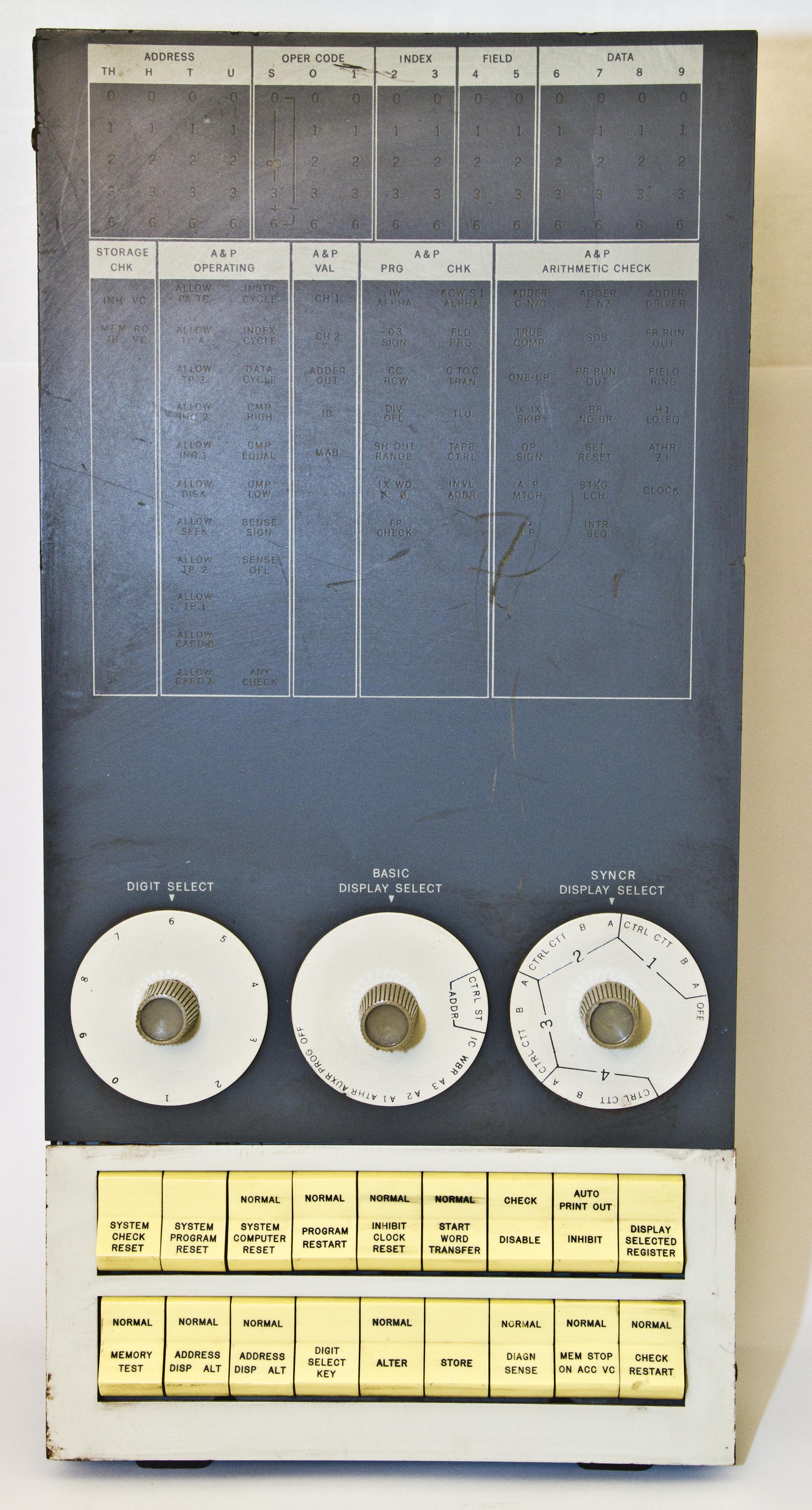
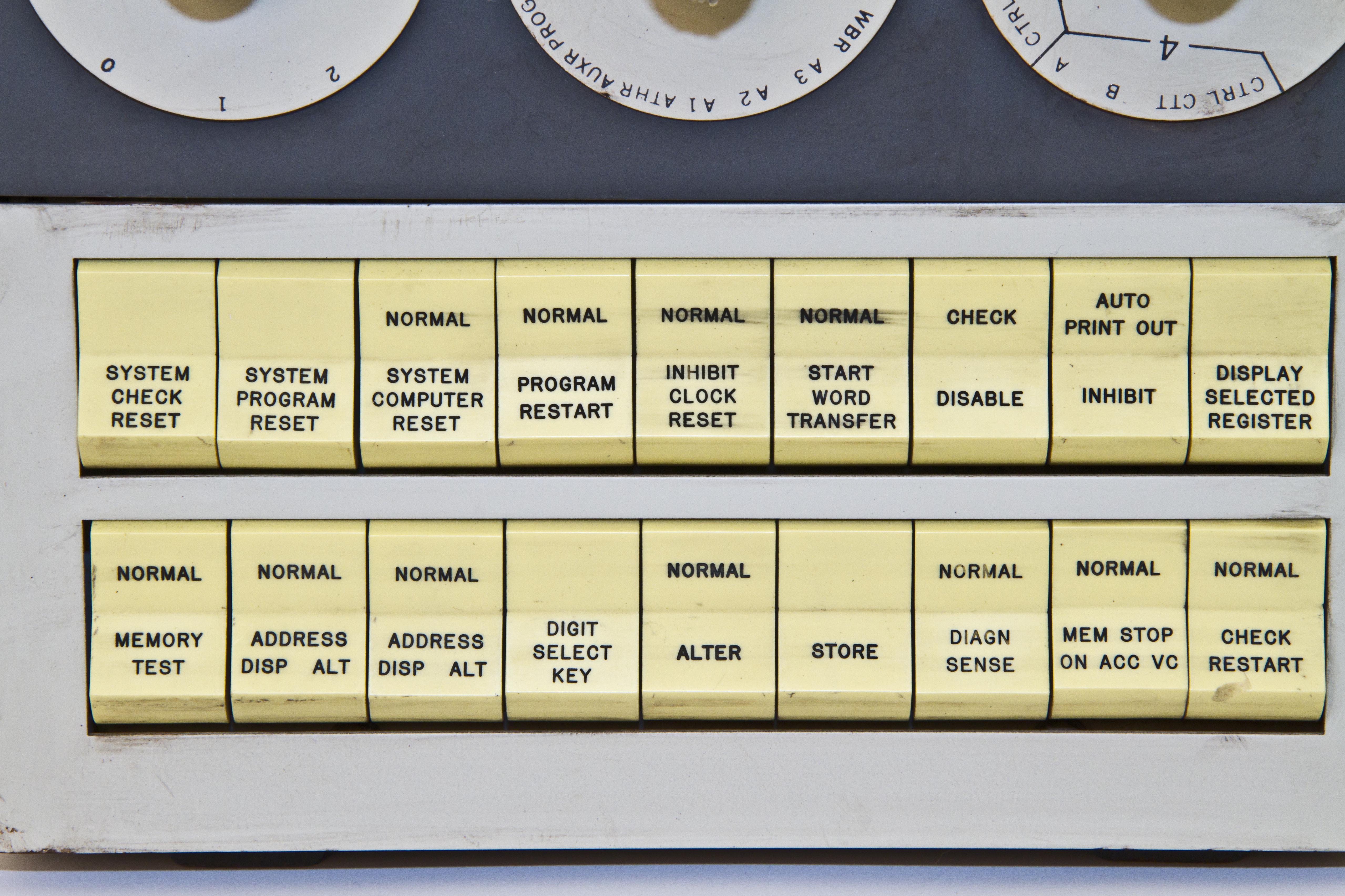
The IBM 9020 system was a specially configured multiprocessor system that was used as the main FAA air traffic control computer from 1971 until the early 1990's. It was installed at the 20 FAA regional ARTCCs (Air Route Traffic Control Centers). Unlike standard IBM mainframes of the day, the 9020 was programmed to operate in "real time": that is, to compute and generate results as fast as or faster than data were fed into it. A full 9020 system consisted of six System/360 mainframes coupled to air traffic controllers' consoles, with data fed into the system from long-range radar and other ground stations. The six System/360 mainframe computers were connected together in a highly redundant and reliable multiprocessing configuration with special I/O capabilities (such as attaching radar consoles) not found in the standard System/360's. Only 25 9020 systems were ever built.
Early 9020 versions used System/360 Model 50 processors for all six processors, but our console comes from the latest 9020E version which used three Model 65's for "compute elements" and three Model 50's for "I/O control elements". Our control console is from one of the Model 65 computers, and is slightly different than the standard Model 65 console.
A quick deviation to discuss the IBM System/360. While technically obsolete now, the introduction of the System/360 family was a seminal event in computer evolution. The instruction set architecture was the most modern for its day and had many influences on current architecture (such as 8-bit bytes and 32-bit words). It also introduced a new I/O approach: a high-performance and programmable "channel" that could attach a vast and diverse set of I/O devices. The most significant feature was the concept of a family of computers, all having the same instruction architecture but with different performance and capacities, and all using the same I/O devices. Initially six models were announced: the Model 30, the Model 40, the Model 50, the Models 60 and 62, and the Model 70. These covered a performance range of about 100:1 and ranged from microprogrammed eight-bit datapath to hardwired 64-bit datapath. Yet they all ran the same software and used the same physical I/O devices.
Another eight model types were delivered during the System/360's lifetime, including the highly influential Model 67, Model 85, and Model 91. As a result of the technical features and especially the scalability and software compatibility across the family, the System/360, and its follow-ons such as the System/370 family, dominated the mainframe business.
The 9020 system had an abnormally long lifetime; the corresponding System/360 commercial products were withdrawn from sales in 1977, but the 9020 lingured in use until the early 1990's. One reason for this long life is the fact that much of the air traffic control application was written in System/360 assembly language. Another factor is the 9020's specialized radar console interfaces. As an example of the 9020 staying power, here's a scary NTSB report from 1996 about ARTCC outages pointing out that some of the ARTCCs are still using the 9020's at late as 1995! This reports discusses problems such as aging components where "replacements can be obtained only by scavenging parts from the [FAA] training computer". Thirty years is a long time for any complex equipment to remain functional, but in the world of computing technology, thirty years is many many generations of architecture and technology. Consider, as one example, that the 9020's used magnetic core memory and that a Model 65's performance was less than 1 MIPS!


I love IBM card equipment!
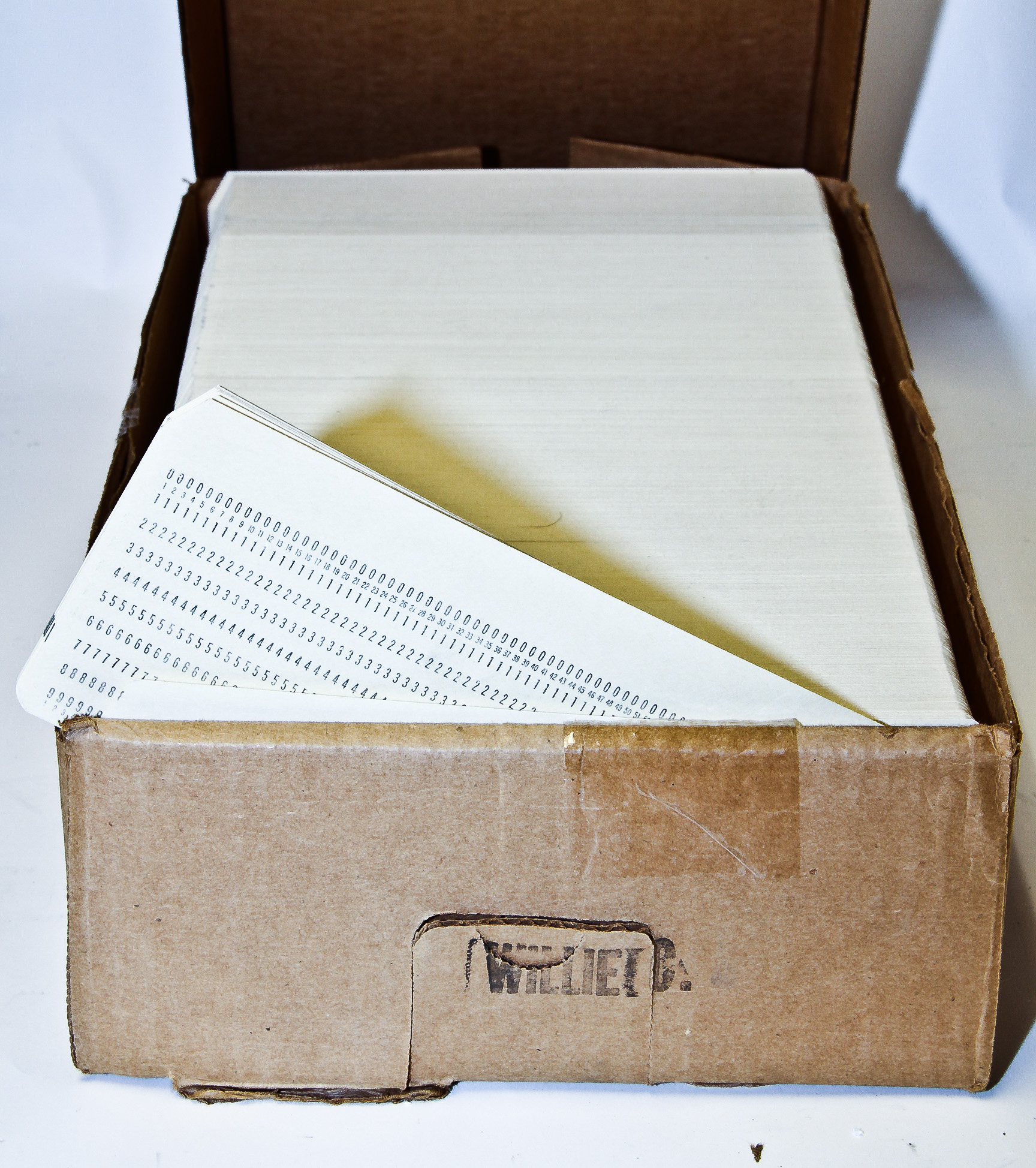
Until the early '60s, most business applications were done on standalone card processing units (called by IBM unit record equipment by IBM) like the ones in our collection (shown following this topic). Even when computers started to be used, most programming was done on punched cards and all computers had punched card input and output. It wasn't until the middle seventies at IBM that we internally switched from card input to CRT terminals. Figure 1 is a box of 2000 fresh punched cards just waiting for our machines to use. (When I programmed on punch cards at IBM, our programs consisted of several trays of cards, each try containing several of these boxes.)
Standalone card equipment ranged from simple devices like keypunches to primitive computer devices like the IBM 602 Calculating Punch which could do multiplication and division. All but the simplest card equipment could be "programmed" by wiring a control board like the ones shown here (often called a plugboard). Other than the fairly rare calculating punches, the most advanced card devices were accounting (also called tabulating) machines like the IBM 407 which read cards and printed a report based on the card data using some counters and simple branching logic (as defined by the plugboard program). These tabulating machines were the computers of their day and were pervasively used in business.
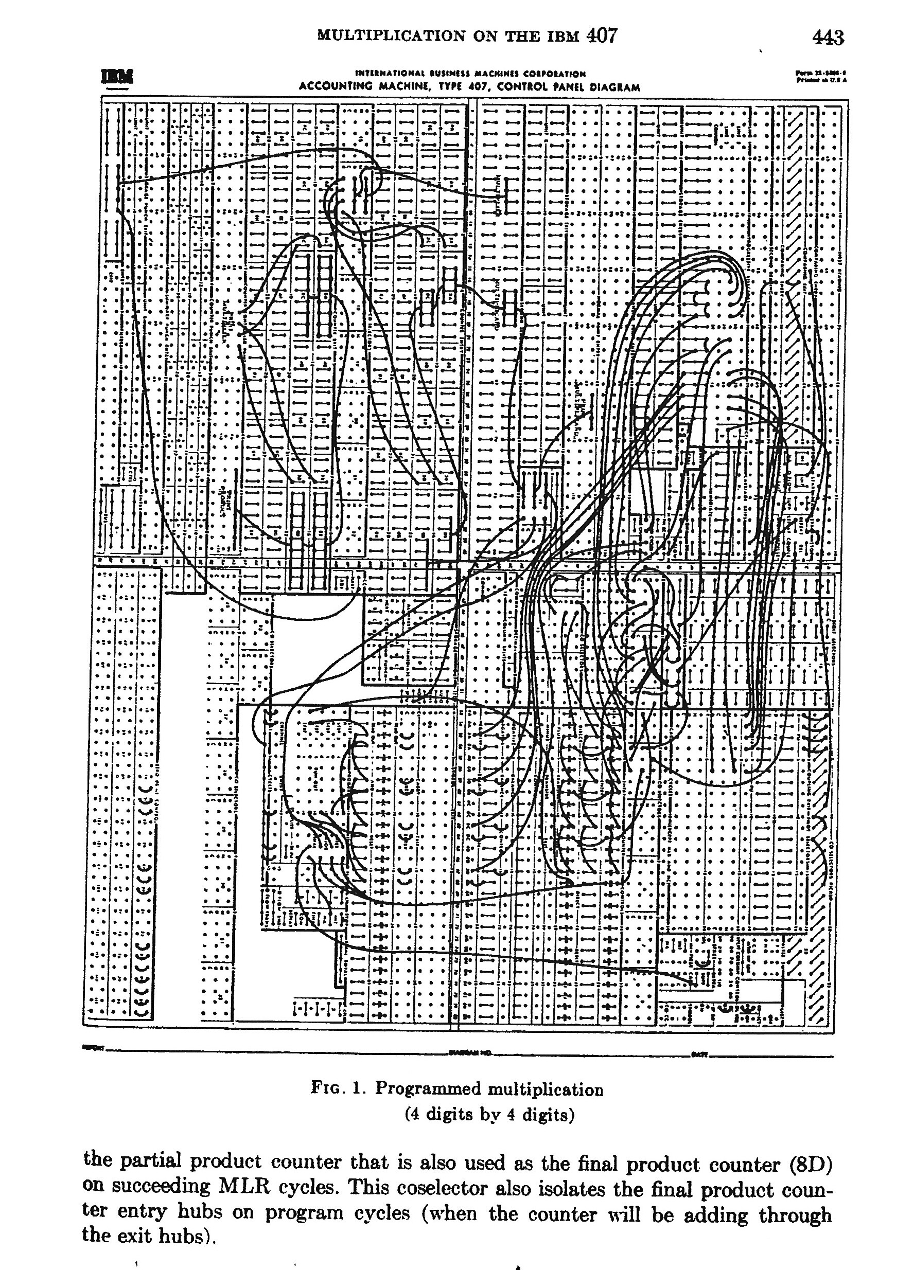
Accounting machines could also be used in non-obvious ways; in my first computer job in 1963 (application programming an IBM 7090 in Fortran and assembler), one of the scientists had programmed an IBM 407 to do matrix multiplication. (Here's a technical paper on this magic. Figure 2 shows a page describing the programming.) Later in college (1965-67) the computer we used (an IBM 1620) had only card input and card output. The output punched cards were hand carried from the computer to the 407 for listing. (The 407 was also used for many business tasks such as producing the student grade reports.) So, since every run I made ended up on the 407, I naturally learned how to program the 407 to do "cute", but useless things. We had lots of 407 boards, each preprogrammed with a particular application, similar to having multiple computer programs today.
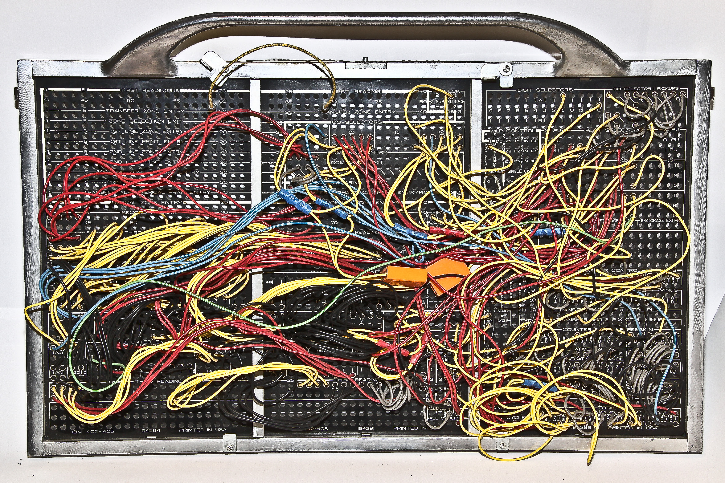
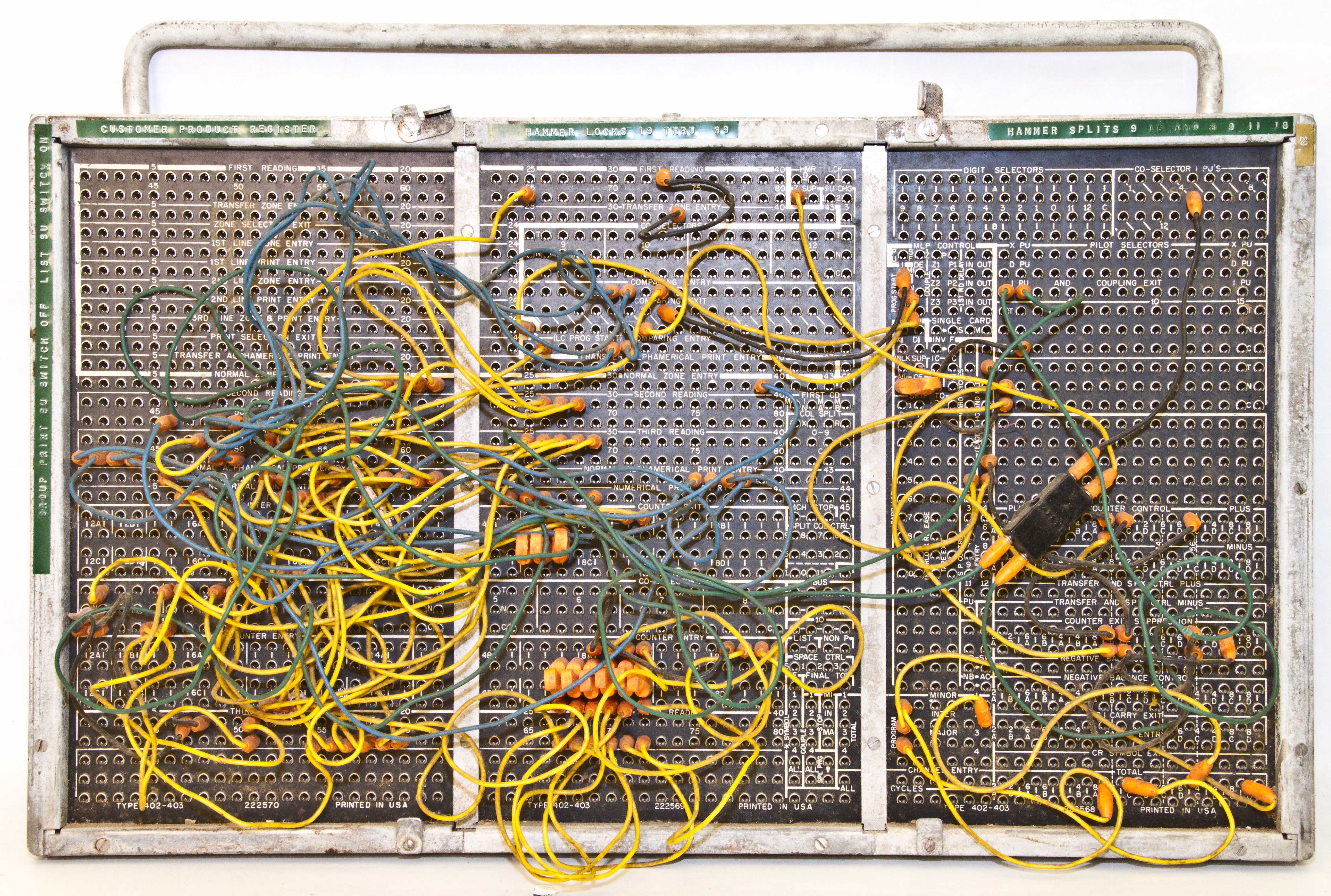
Here is my collection of plugboards for IBM card equipment. Figure 3 is the board for an IBM 402 accounting machine, an earlier version of the 407, and Figure 4 show how the plugs come out of the other side.
When the plugboard is inserted into the machine, the plugs contact sockets that are hardwired to card read brushes, card punch controls, and internal counters and other logic.
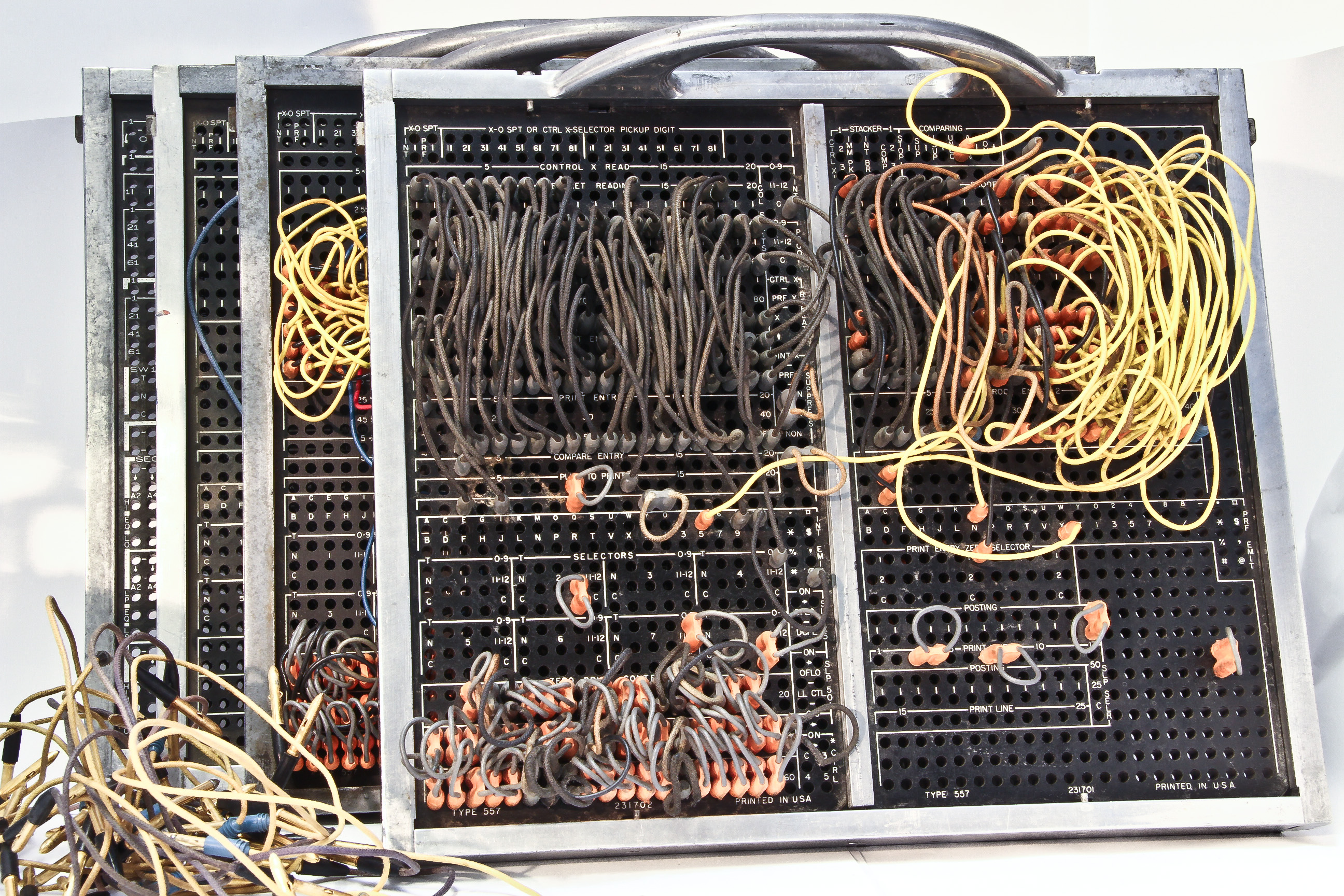
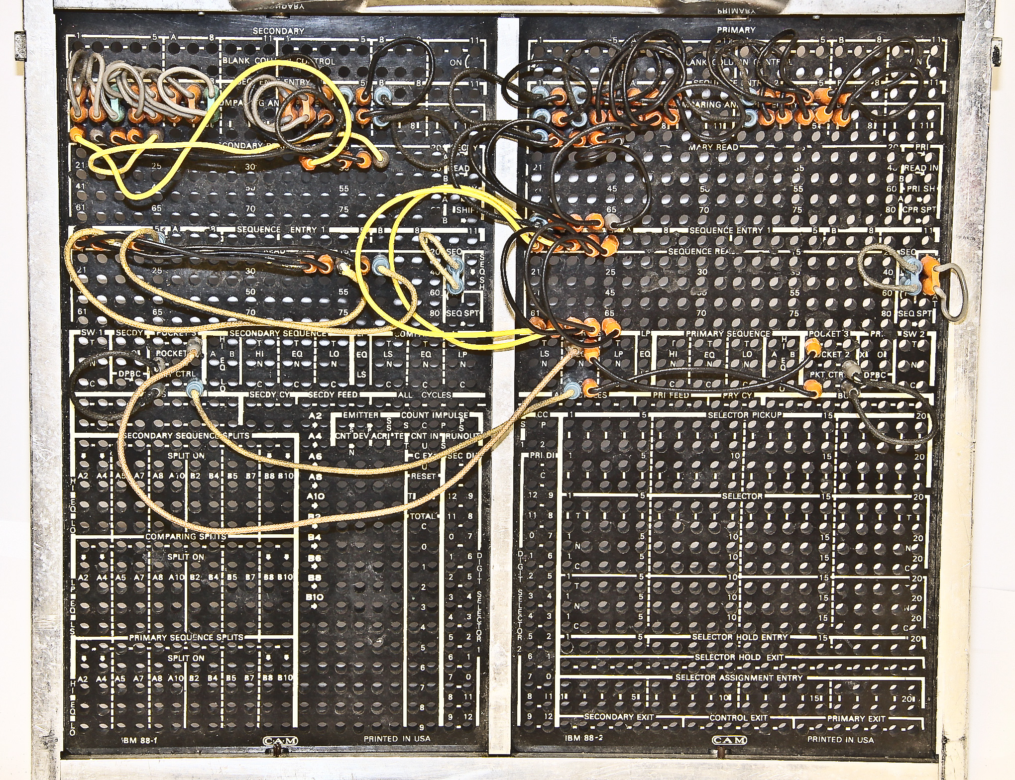
Figure 4 also shows the label of what this program supposedly did (payroll). Figure 5 shows our four IBM 557 Alphabetic Interpreter plugboards. Since we actually have a 557 in the museum, having multiple boards allows us to have different programs ready to us. On the left side are some programming "statements" (plug wires) ready for more programming.
Figure 6 shows the plugboard for an IBM 088 Collator. Figure 7 shows the plugboard for an IBM 533 Card Read Punch. The 533 is particularly important as it was the input/output device for the IBM 650 computer, commonly considered to be the first mass produced computer. The 650 was the first computer I ever saw in person (on a high-school field trip to the engineering lab at UC, Berkeley), and it had a great influence on my later choice to specialize in computers.
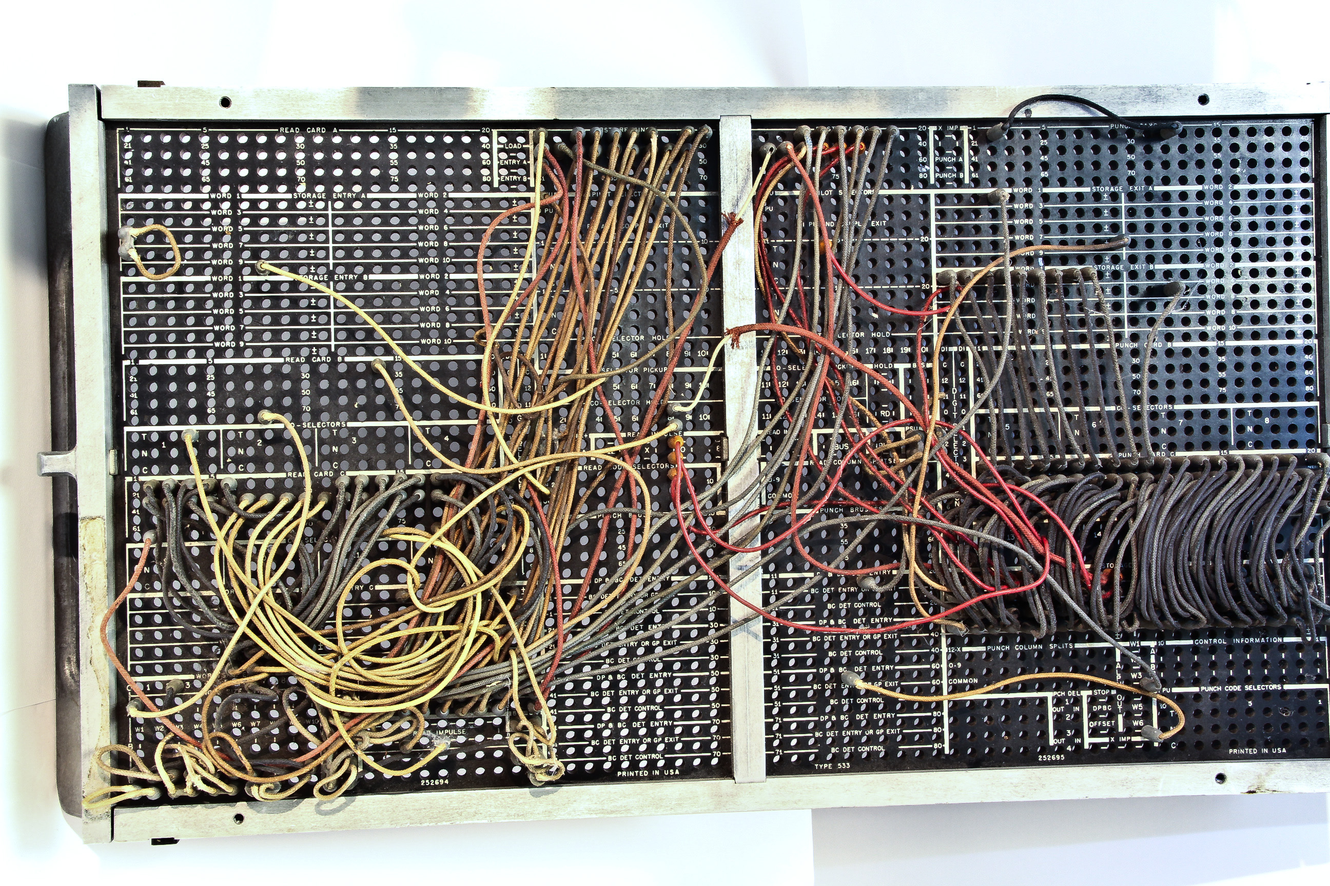
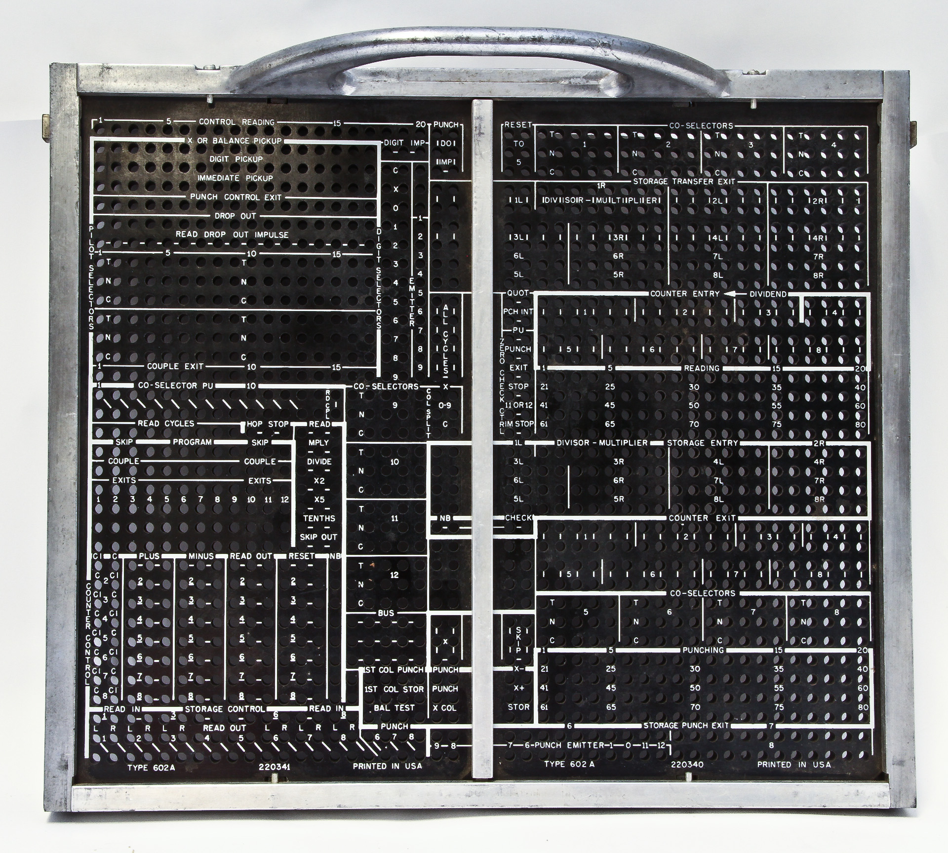
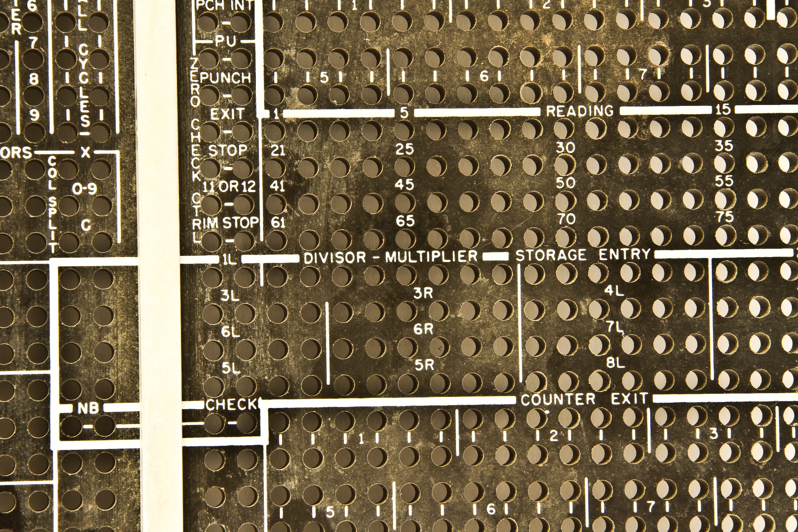
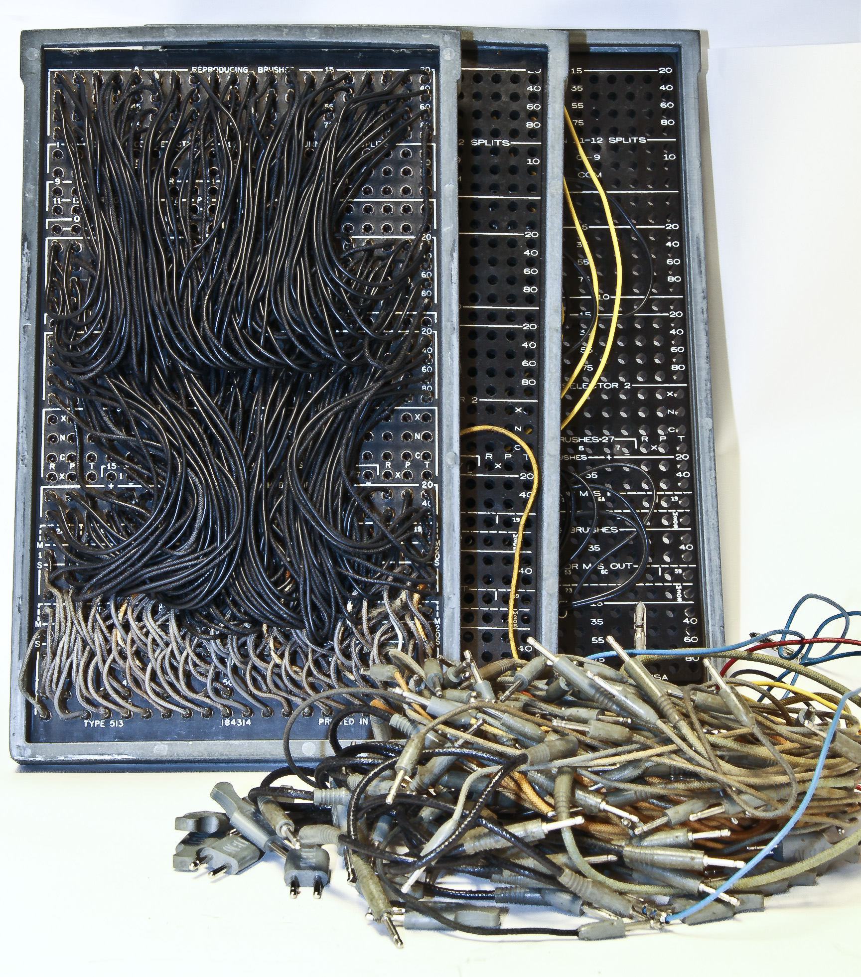
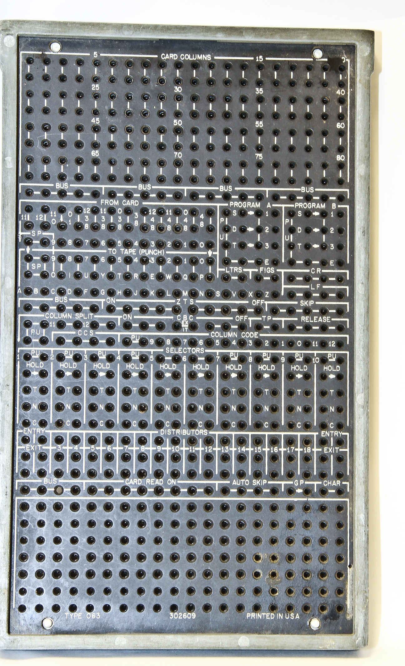
Figure 9 shows the plugboard for an IBM 602 Calculating Punch. Figure 8 is a closeup of this board showing some of the controls for multiplying and dividing. Figure 10 shows our three plugboards for our IBM 514 Reproducing Punch. (Also shown are some programming plugs; these can be used on all the IBM boards.) Figure 12 show the control board for a rare device: the IBM 063 Card-Controlled Tape Punch. This device read cards and punched the corresponding values in paper tape.
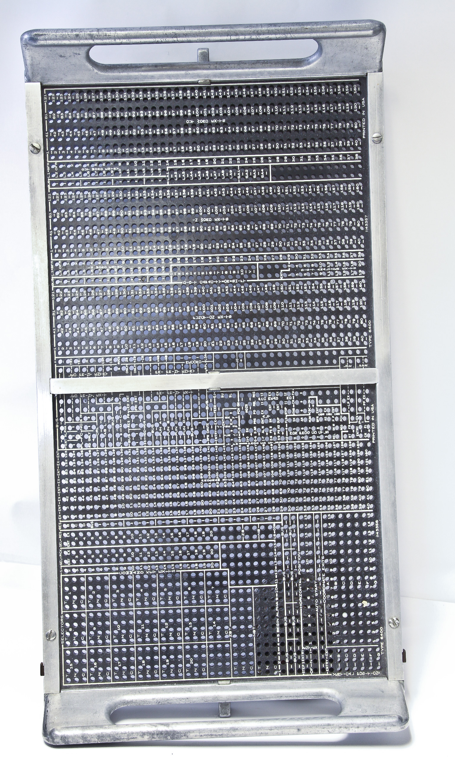
Finally, Figure 11 shows a particularly rare piece: the control plugboard for an IBM 6400 Accounting Machine. This device is little know and I've never seen one (as opposed to all the other devices discussed in this section).
Figure 13 shows a new variety of a 402-403 control board. Note that Figure 3 shows our other 402-403 board and this new one is subtly different. Figure 14 shows a newly arrived control board for an IBM 85 collator. The model 85 is an earlier collator version that the Model 88 whose control board is shown in Figure 6. Note that the 85 board is much different (simpler) than that for the 88. It seems that every different version of the same type of device (collator, interpreter, etc.) had a different control board.
Finally, I now possess a IBM 407 control board. As described above, this is my favorite card devices and the epitome of card processing complexity. Figure 15 show the large (and heavy, about 25 pounds) 407 control board with an apparently working program. Figure 17 shows the label of the program which is "PAYROLL/CALC FICA/RETIREMENT/TAXABLE WAGES". This payroll application is a typical 407 function (our college 407 was used monthly for this very purpose). Figure 16 shows a close-up of some of the program's logic. The big orange and gray blob things are splitters and combiners of signals.
I'm getting too many of these to photograph them, so here is my inventory of IBM card equipment control panels:
Two general types of memory were used in computers before magnetic core memory was used: CRT or Williams Tube memory, and Delay Line memory. We have an example of CRT memory in the Components section of the museum. Delay line memories differed in the type of delay medium, but all used the same general principle of representing bits as mechanical "waves" in some media, creating them at one end of a "wire" reading them as them arrive at the other end, and recirculating the data back to the start of the wire. The stored data thus consists of bits (as mechanical waves) flowing around and around a loop containing a medium for propagating the bits. The length of the loop and the frequency of the mechanical waves determine the storage capacity.
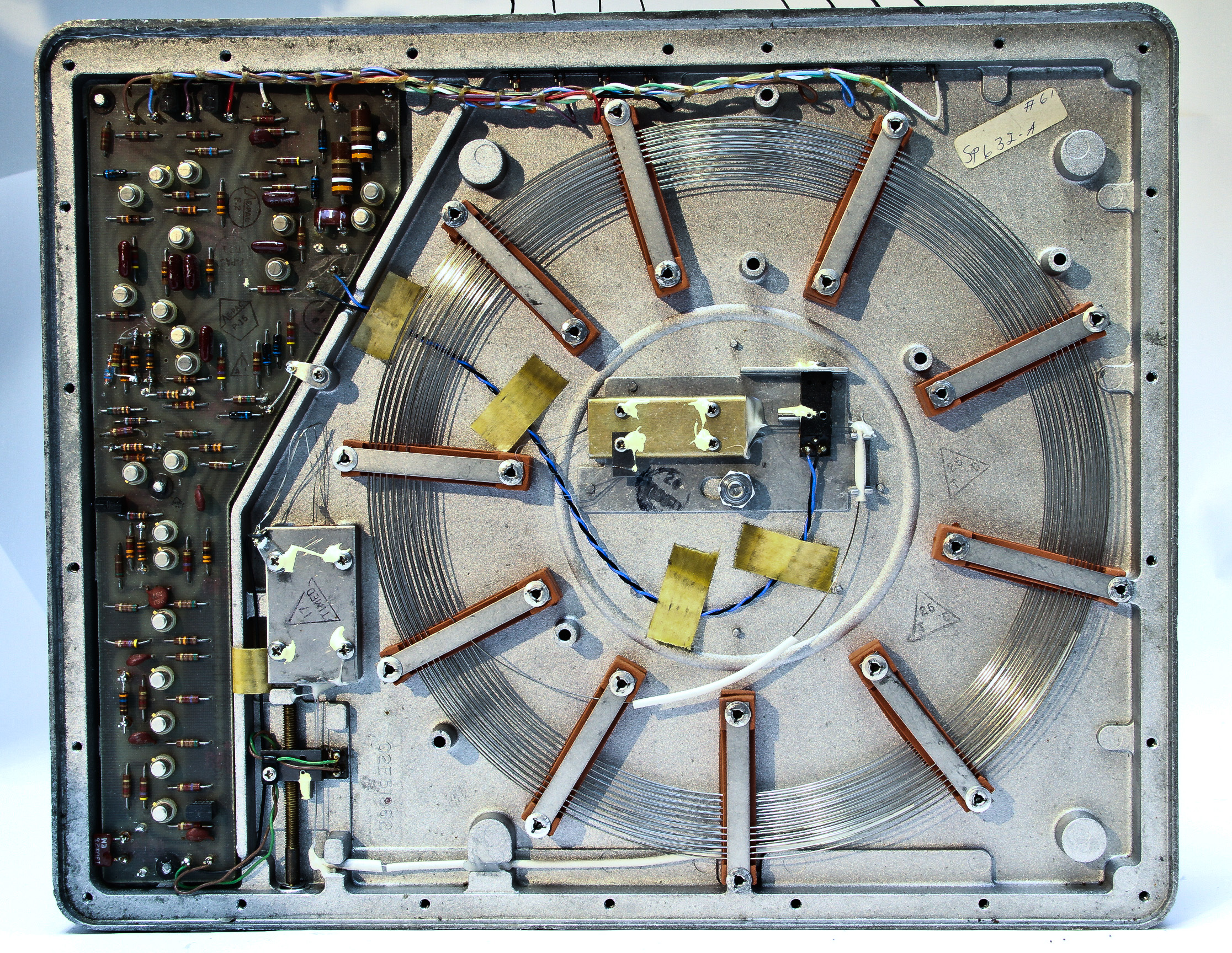
Mercury tubes were first used for delay lines; for example the UNIVAC I used mercury delay lines. A major improvement over mercury tubes was Magnetostrictive memory. The museum has a great example: it is the memory from an IBM 2848 control unit which fed video data to several IBM 2260 Display stations, the first video display terminals that IBM made (shipped in the mid-1960's)
Magnetostriction means that a material (a metal wire in our case) changes shape in the presence of a magnetic field. In our case, the wire expands or contracts , thus creating a mechanical pulse that propagates along the wire. Our wire was made of a special nickel-titanium-iron allow that had the right properties for propagating the mechanical impulse along the wire.
Figure 1 shows a memory module from the 2848 control unit. Each module held 11,520 bits, and there were up to four modules in a 2848 control unit, which could service eight 2260 terminals. A 2260 screen was 12 rows of 80 characters. Each character was represented by a six-bit code, so a 2260 needed 5,760 bits to refresh its display.
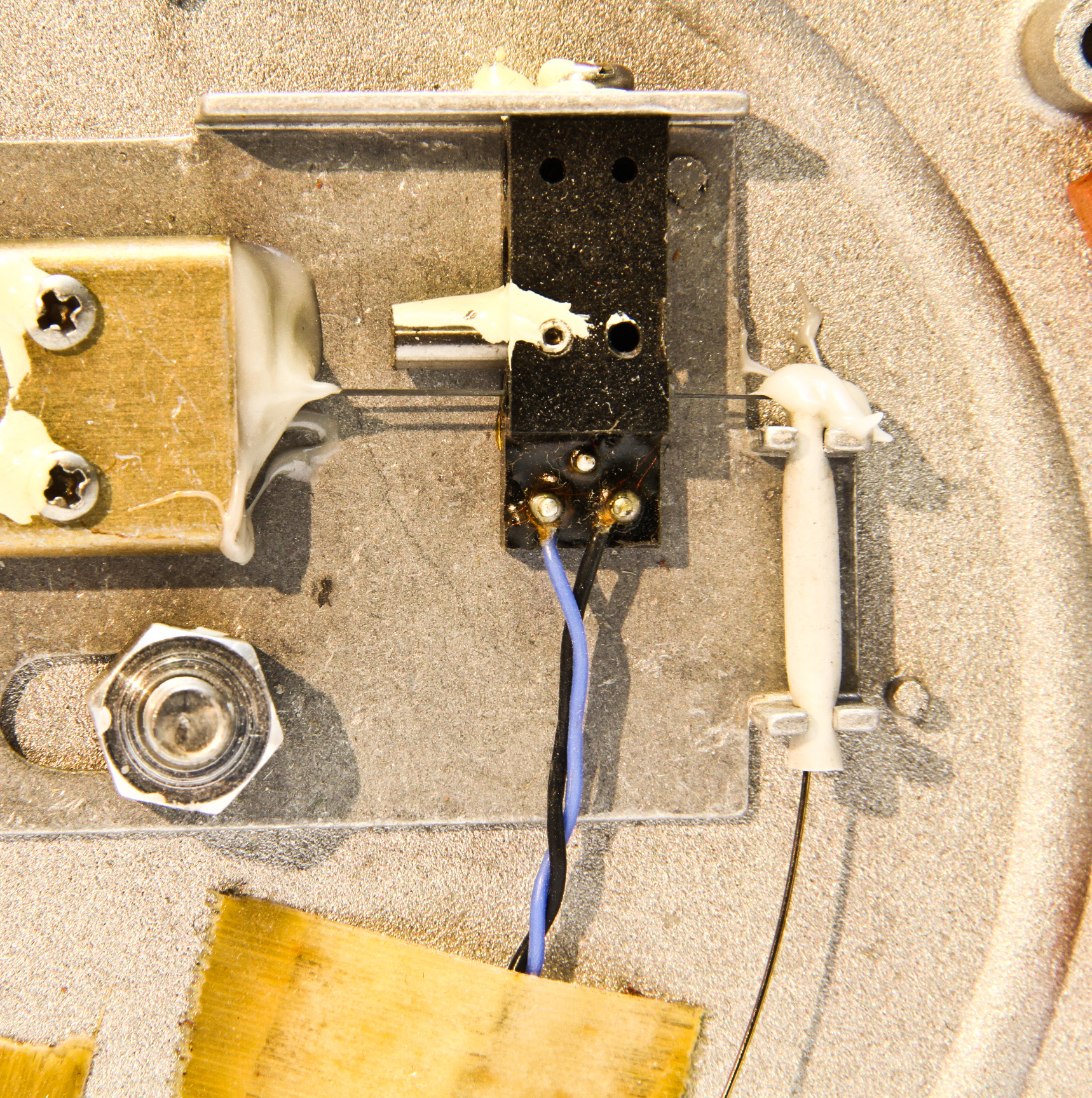
The memory worked by generating "bit" waves using a magnetic transducer at one end of the storage wire. Figure 3 shows the transducer and start of the wire, and Figure 4 shows the end of the wire, the sensor, and a fine-tuning adjustment. Figure 2 shows a close-up of the wire coils of wire, as well as the circuit board which used discrete germanium transistors. The access time for this memory was about several hundred microseconds, the time for a wave to travel along the complete wire. Both ends of the wire are dampened to prevent feedback of reflected waves.
In its heyday of computer design, IBM not only had great electronic technology but their packaging was unbelievably good. Here are some examples in the museum.
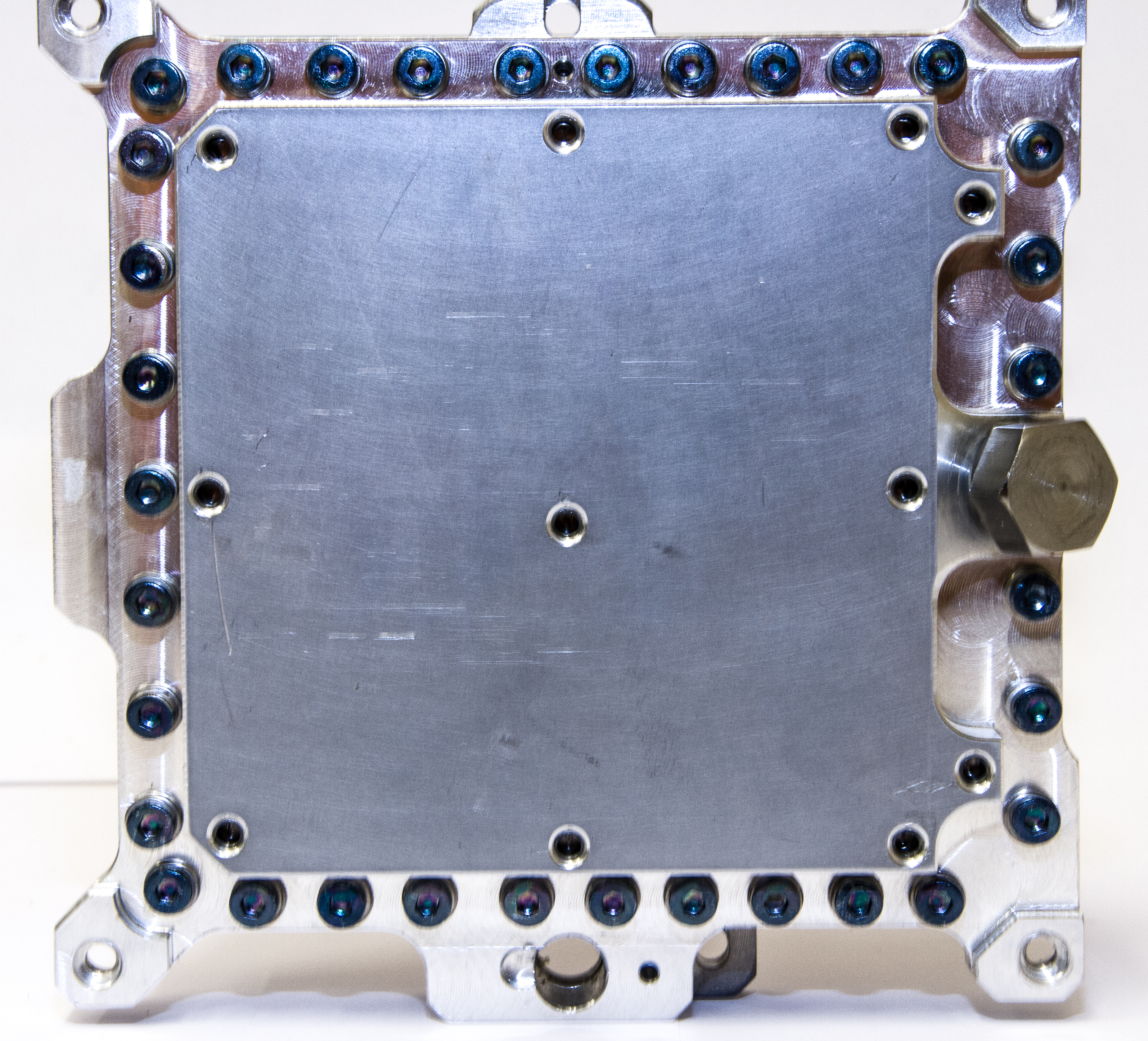
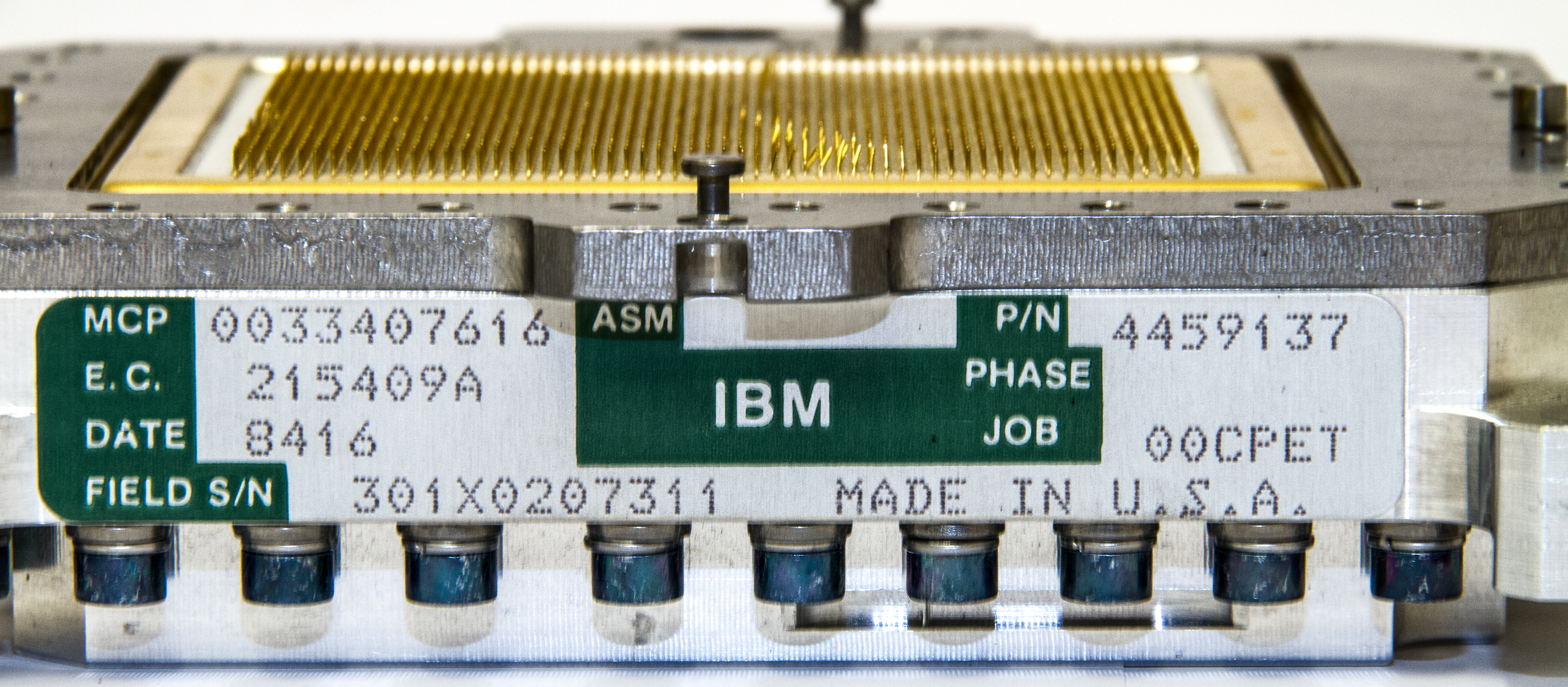
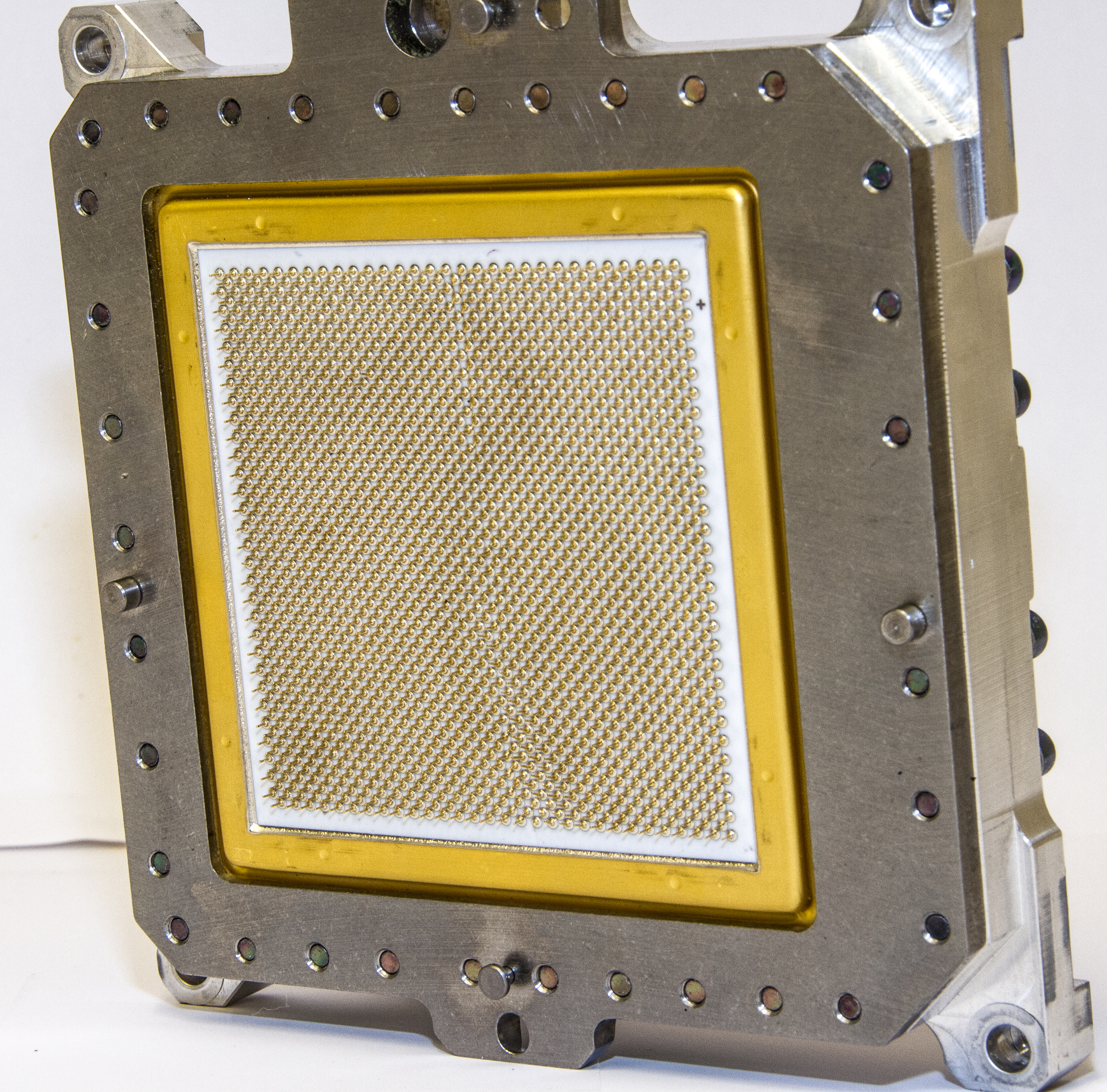
Figures 1-5 shows the IBM TCM used in the 3081 computers, circa 1981. It is six inches square and weighs about 5 lbs. The outside of the cover is shown in Figure 4. The reverse side of the cover is Figure 1 which contains an 11x11 array of spring-loaded copper slugs. Figure 5 shows a side view of the cover and slugs (I have lost some of the springs so some of our slugs don't pop-up). When the cover is mounted on the bottom assembly, the copper slugs each press one one of 11x11 flip-chip mounted gate-array TTL chips, each containing about 704 circuits. The chips are mounted on a thick ceramic substrate containing 33 wiring levels. The back side of the ceramic, shown in Figure 2, contains 1800 I/O pins.
The area above the copper slugs in the cap was filled with helium to help conduct heat to the cover. The cover was attached to a water cooled plate.
Okay, so this is not exactly an old item: it was shipped in 2006. It does, however, show another instance of IBM's great technology capability, so since I'm covering older technology I thought it belonged—it's just so cool!
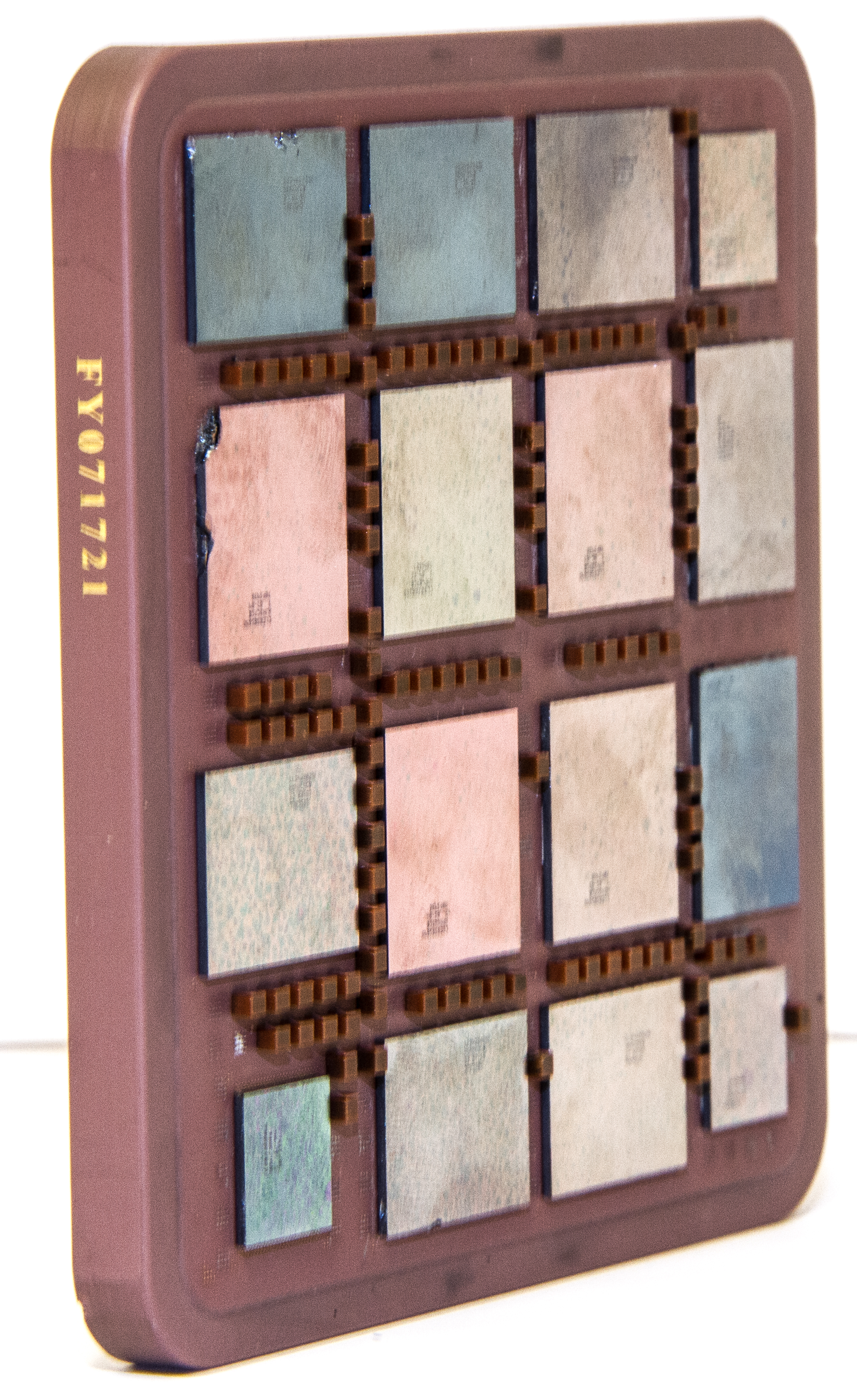
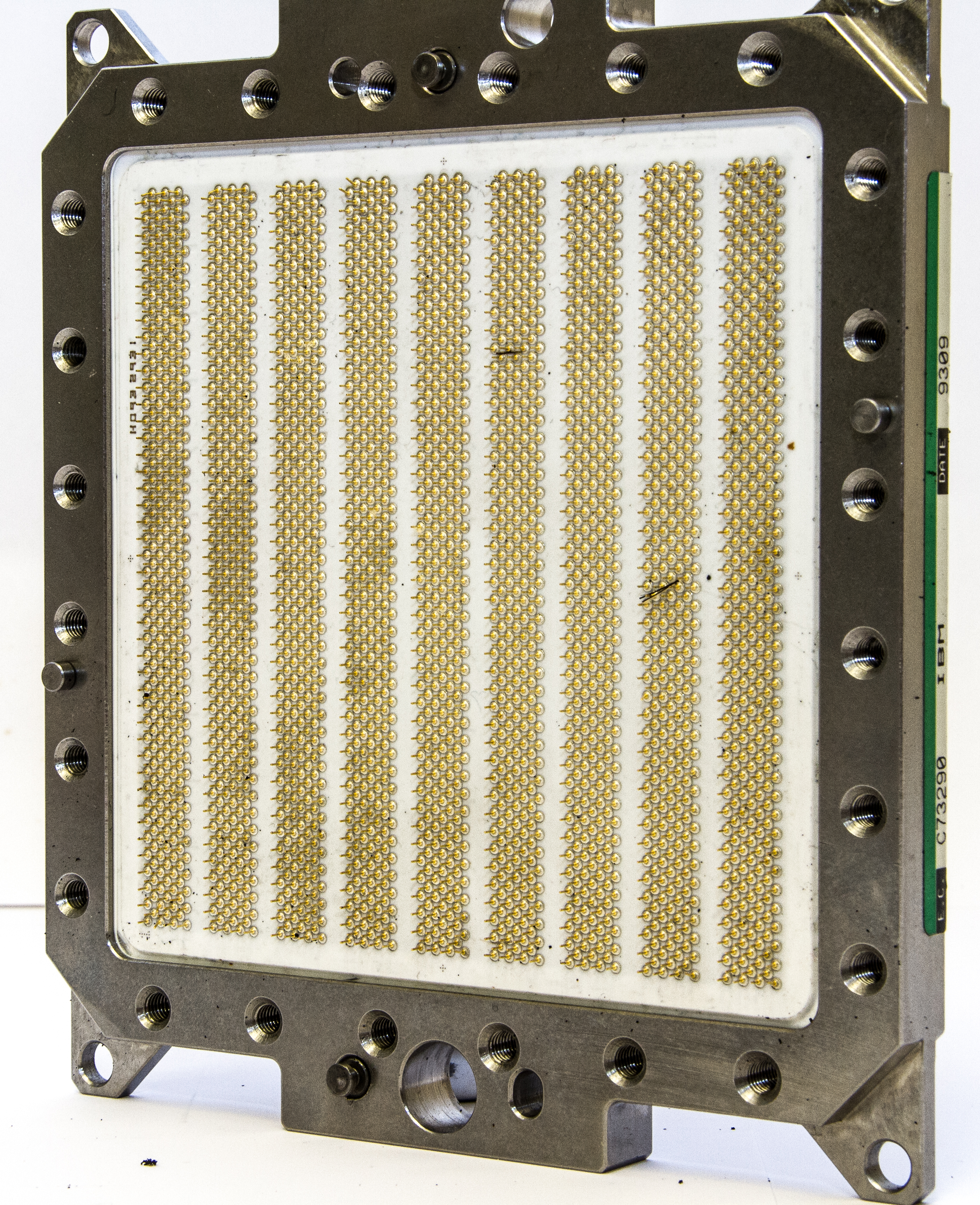
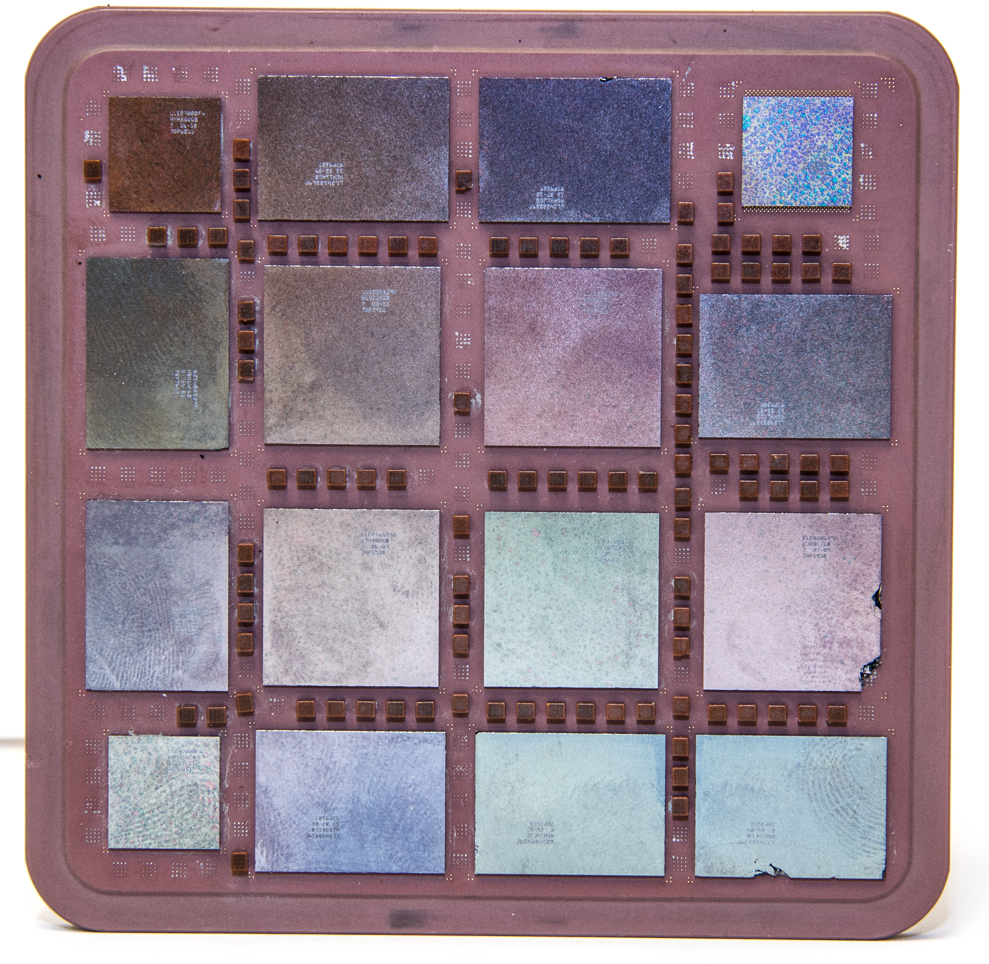
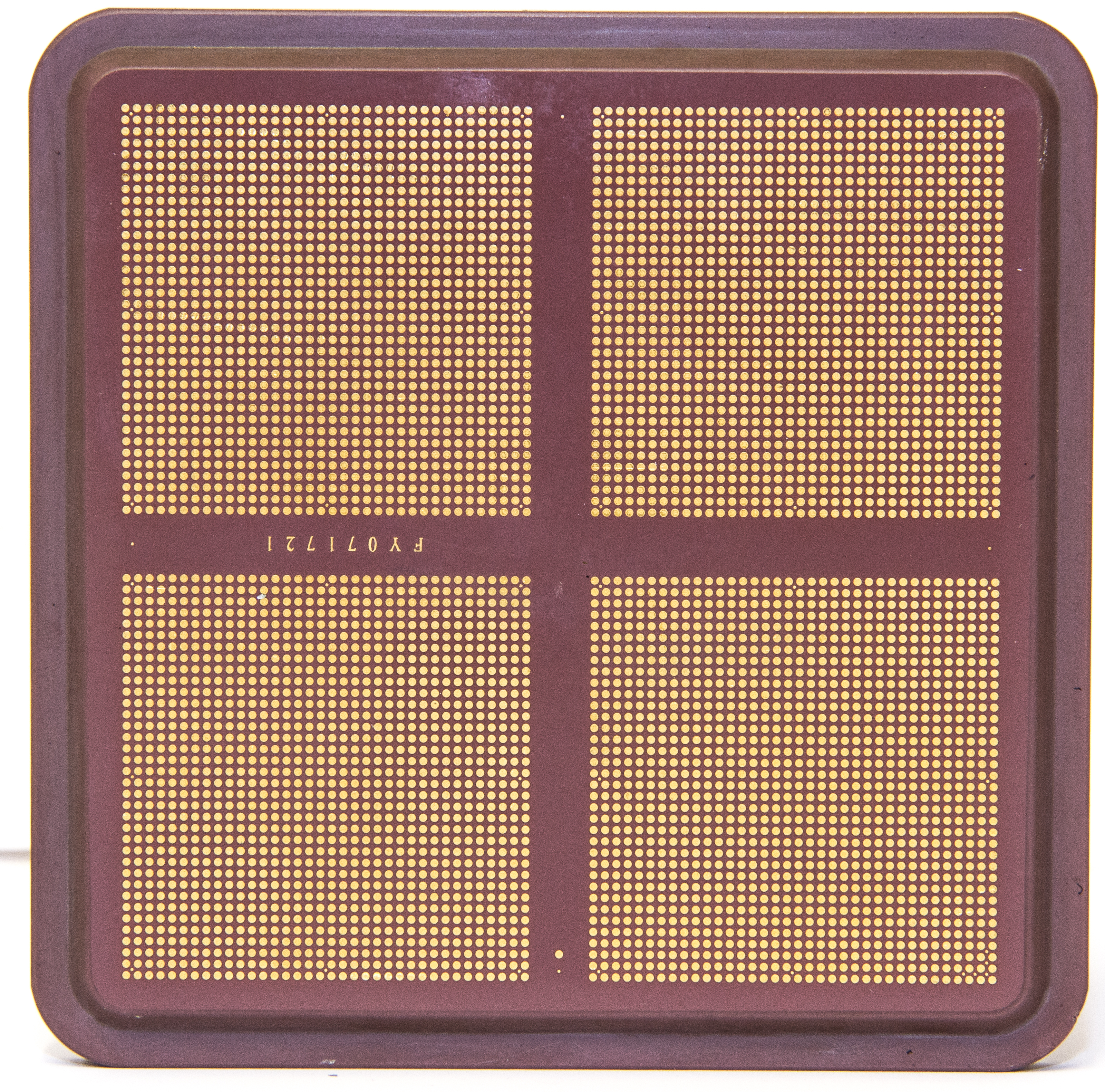
This is a processor module from the IBM Z9 mainframe/super server. There are 8 processor chips, each containing 2 cores, each with 256KB of L1 cache, along with 4 L2 cache chips comprising 40MB, plus controllers for cache, memory, and I/O. About 4.5 billion transistors altogether with a very impressive package.
The ceramic package has 102 internal wiring planes, 5,184 total pins including 2,970 signal pins. It dissapates 1200 Watts of heat and is normally water cooled, but there is a air-controlled backup where the clock speed is reduced.
The Z9 chips are implemented in IBM 90nm technology. Interestingly, we used that same technology for a processor design we did in the mid 2000's. Our tiny chip (about 30M transistors) could run at 2.0 GHz. The Z9 processor chips run at 1.7GHz. This is a tremendous achievement considering how much larger the Z9 is than our processor (150x spread across 16 chips!).


JOSS (JOHNNIAC Open Shop System) was a new computer language, which together with new remote terminals, attached to RAND's JOHNNIAC mainframe computer, comprised one of the first time sharing computer systems.
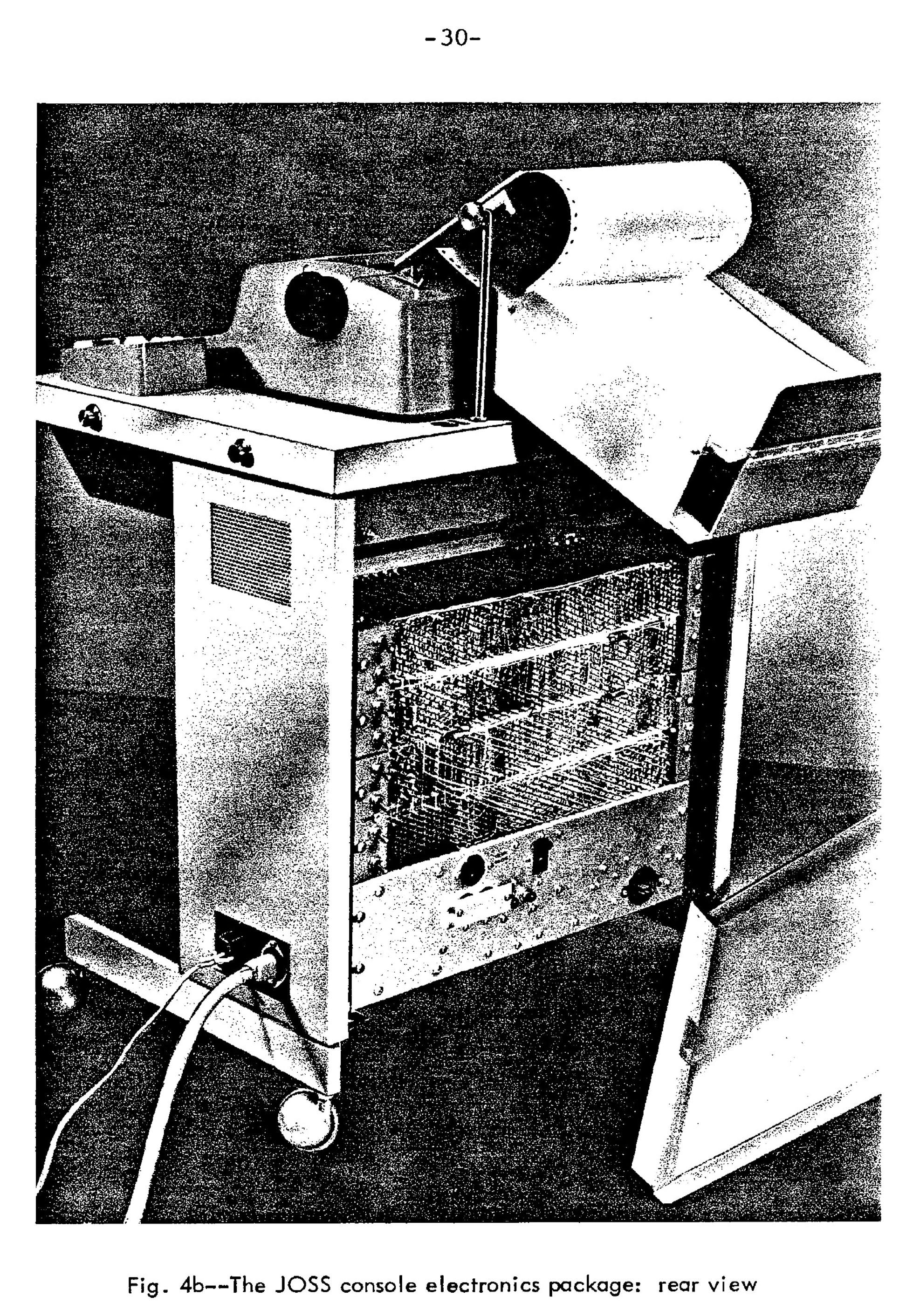
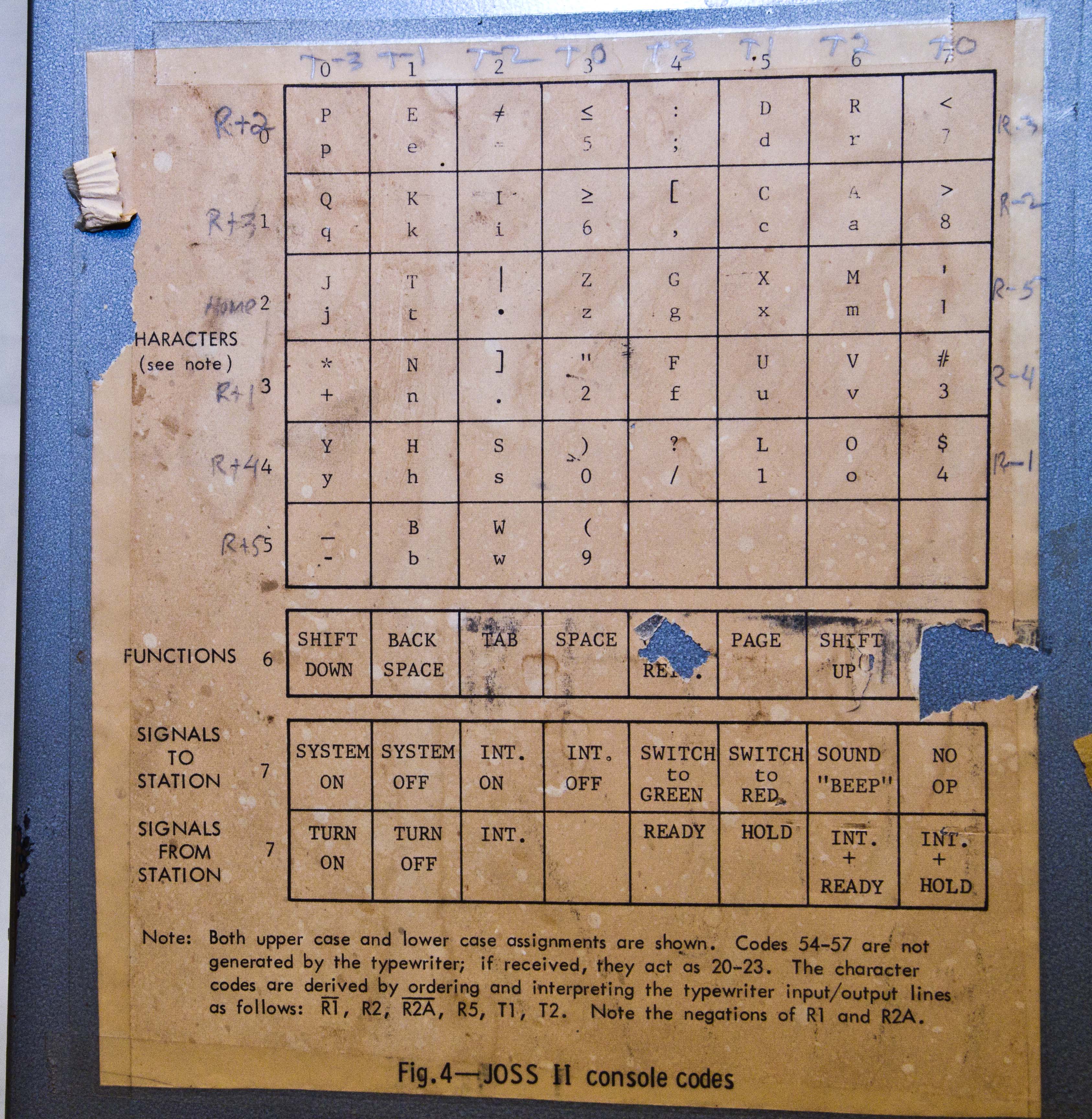
This RAND document from RAND contains more information about the language and using the JOSS system. Of particular interest to us is the special console designed for JOSS, which is described in detail in this RAND report. The JOSS console comprises a modified IBM 731 "input-output" electric typewriter attached to a specially designed control logic which interfaces between the typewrite and a full-duplex communication channel. Figures 1 and 2 come from this RAND report showing the console: the typewriter on top of the control box.
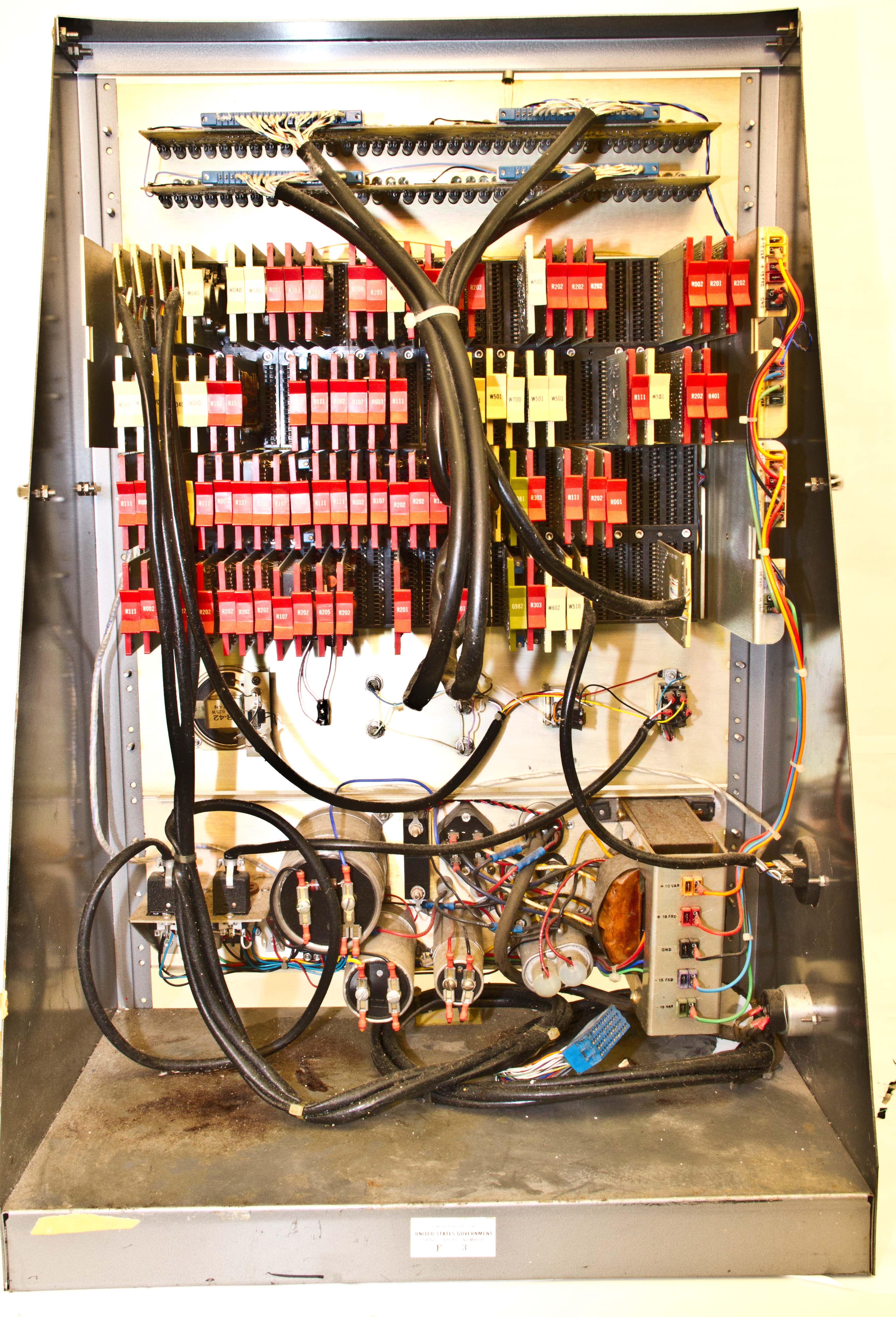
The museum contains an instance of the JOSS console control box. Figures 3 and 4 show the front and back sides. Figure 5 shows one of the 50 cards containing in the control unit's logic. This appears to use diode logic. Also in Figure 5 we see the RAND label and serial number of our controller. Figure 6 show some information pasted to the side of the controller, and Figure 7 show some of the status lights on the top of the controller.

A keypunch was the source of data and programming when I started in computing. As one typed on he keyboard, the characters were punched into the card (using a unique 12-hole code). After all your data or program lines were punched, the collected cards were read by standalone card devices (like a sorter) or by card readers attached to a computer. As late as the early 1970's at IBM, our programs consisted of thousands of cards held in metal trays (that fit into special file cabinets.) A program library was thus very similar to a real library, only with many trays of cards instead of books.
Much more information about IBM keypunches, history, how they work, codes, and so forth, is found here.
Figure 1 shows our IBM 026 Keypunch. The 026 was first introduced in 1949 replacing even older keypunch models.
Figure 2 shows our more modern IBM 029 Keypunch. The 029 was first introduced in 1964 and was the last version IBM made.
And Figure 3 show a semi-portable (it weighs about 40 lbs.) IBM 010 Keypunch. This device allows the operator to punch one card column at a time (the keys trigger a solenoid punch). Interestingly, I can't find any references to a IBM model "10" keypunch. There is a manual 010 that is similar, but obviously of earlier origin.
The IBM System/360 family was a very significant milestone in computer history. The Model 30 was the smallest member of the family that was fully instruction-set compatible with the other models. The hardware had an eight-bit datapath and the System/360 instruction set was completely microprogrammed along with an emulator for the popular IBM 1401.
The museum has a control panel from a Model 30. Ours is interesting because it has controls not normally found on a Model 30 console. For example, in this picture, note the blank area to the immediate left of the emergency pull" power disconnect (the upper right red button). On our console, this area has controls for what sounds like "expanded storage".
On a personal note, in 1967 and 1968 at IBM, I often used a Model 30 directly and was very familiar with the console.
For more System/360, see our IBM Air Traffic Control Console.
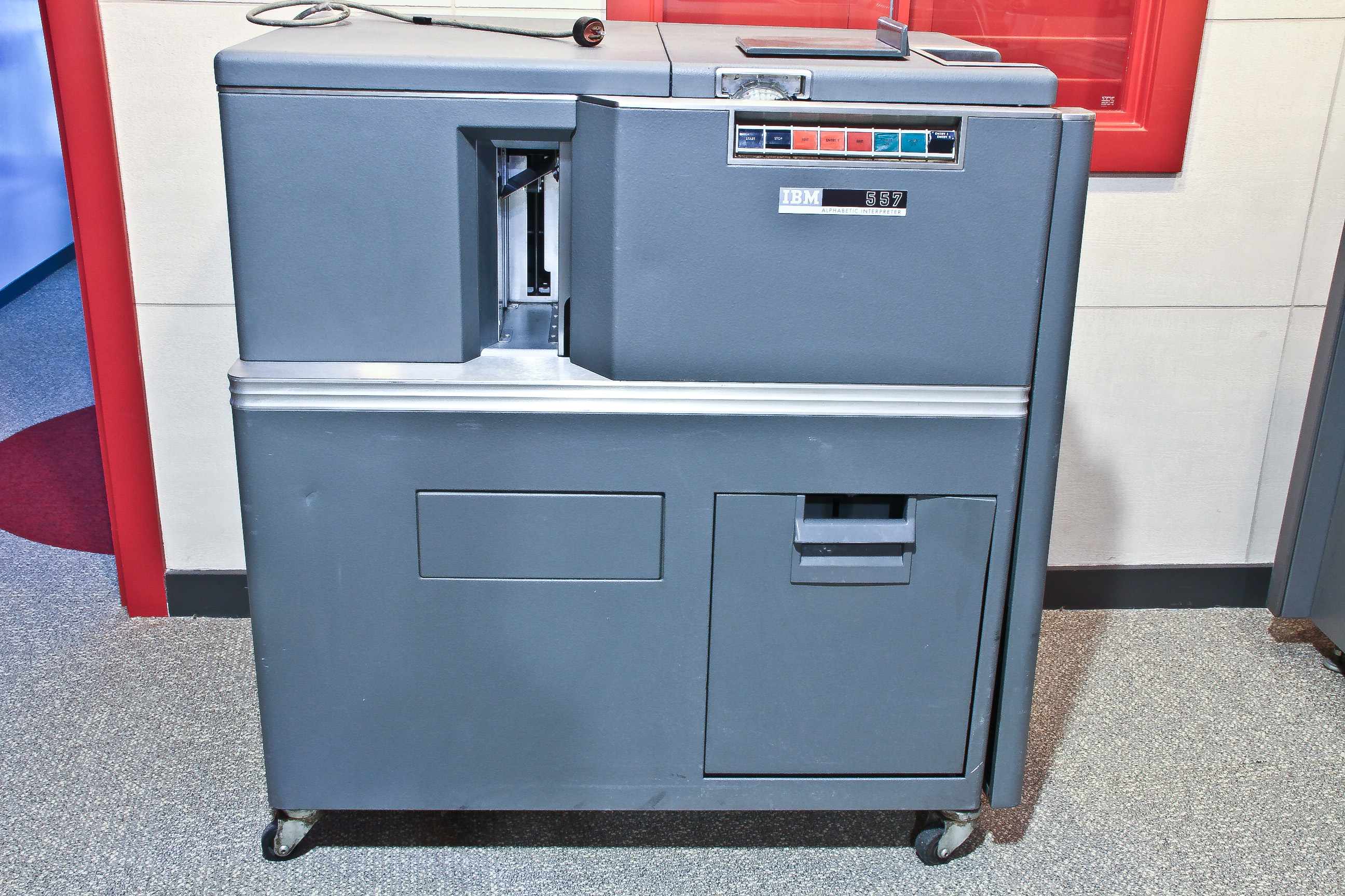
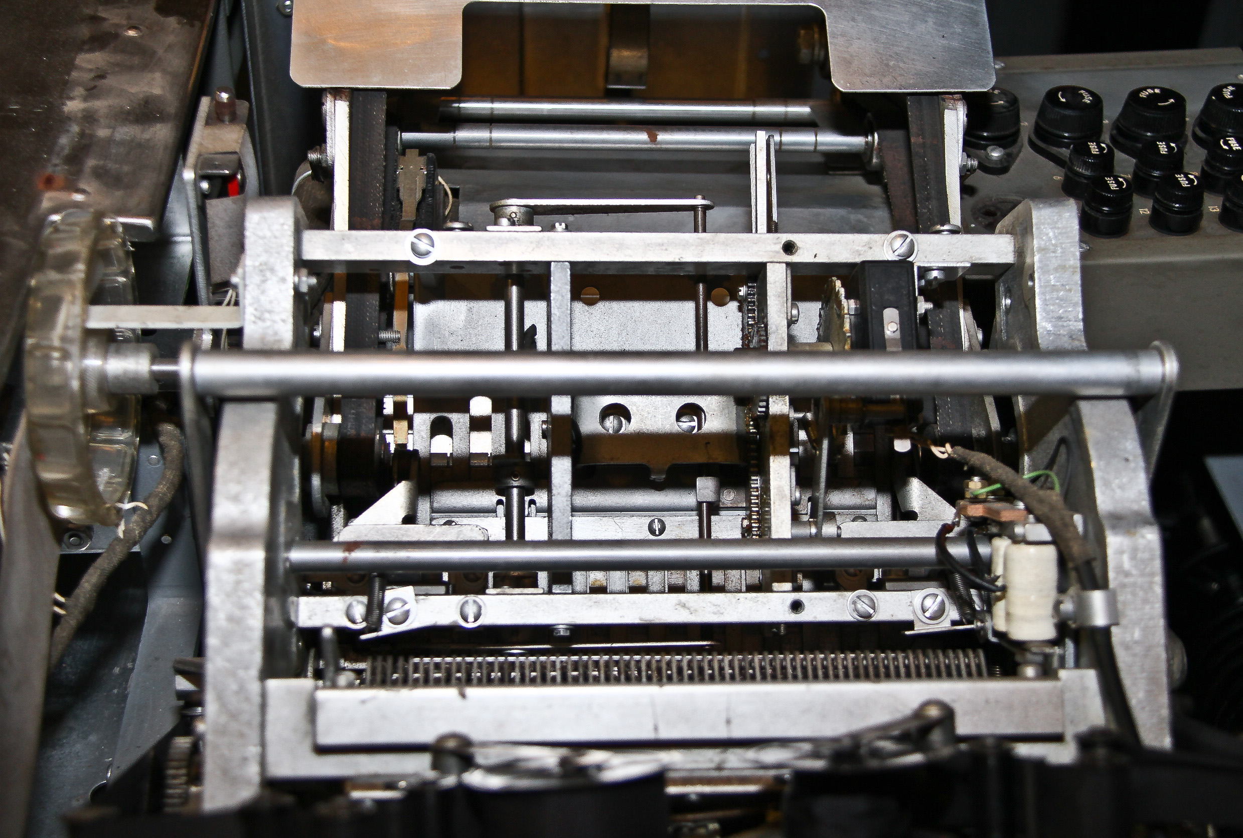
Figure 1 shows our IBM 557 Alphabetic Interpreter. It is essentially a card printer. The information to be printed, however, comes from the same card that is being printed, and the plugboard control can perform reformatting of the data to be printed. This process requires a lot of complicated machinery. Figure 2 shows part of the card path mechanics. Card are read at the top and part of the 60 individual print bars is seen at the very bottom. The 557 was first introduced in 1954 and is the next-to-last of a line of IBM card interpreters.
An example application of the 557 is printing payroll checks on card stock. Another of IBM's card machines (or even a computer) would punch the information on cards, which would then be run through a 557 to print the readable information such as recipient and amount.
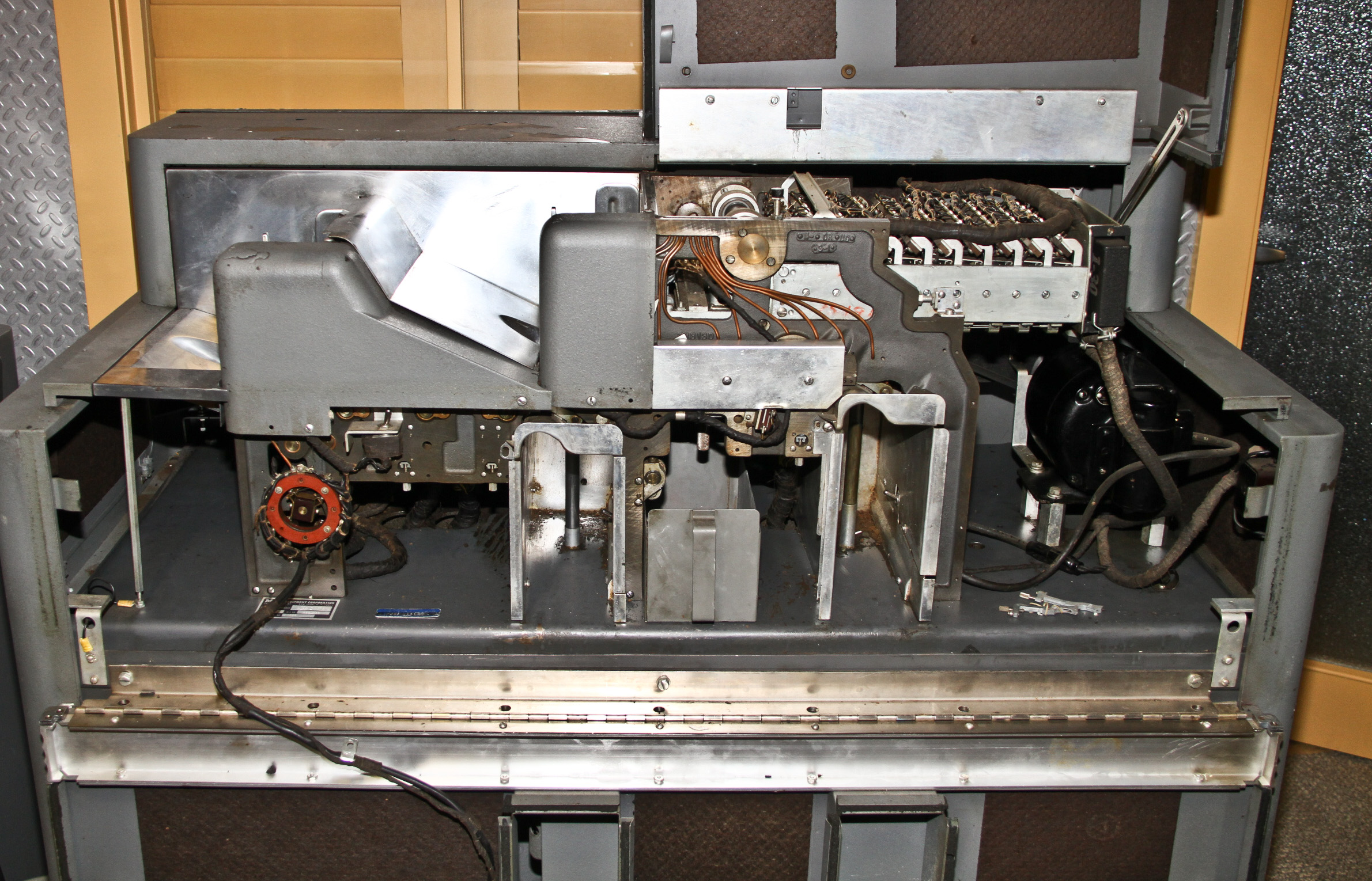
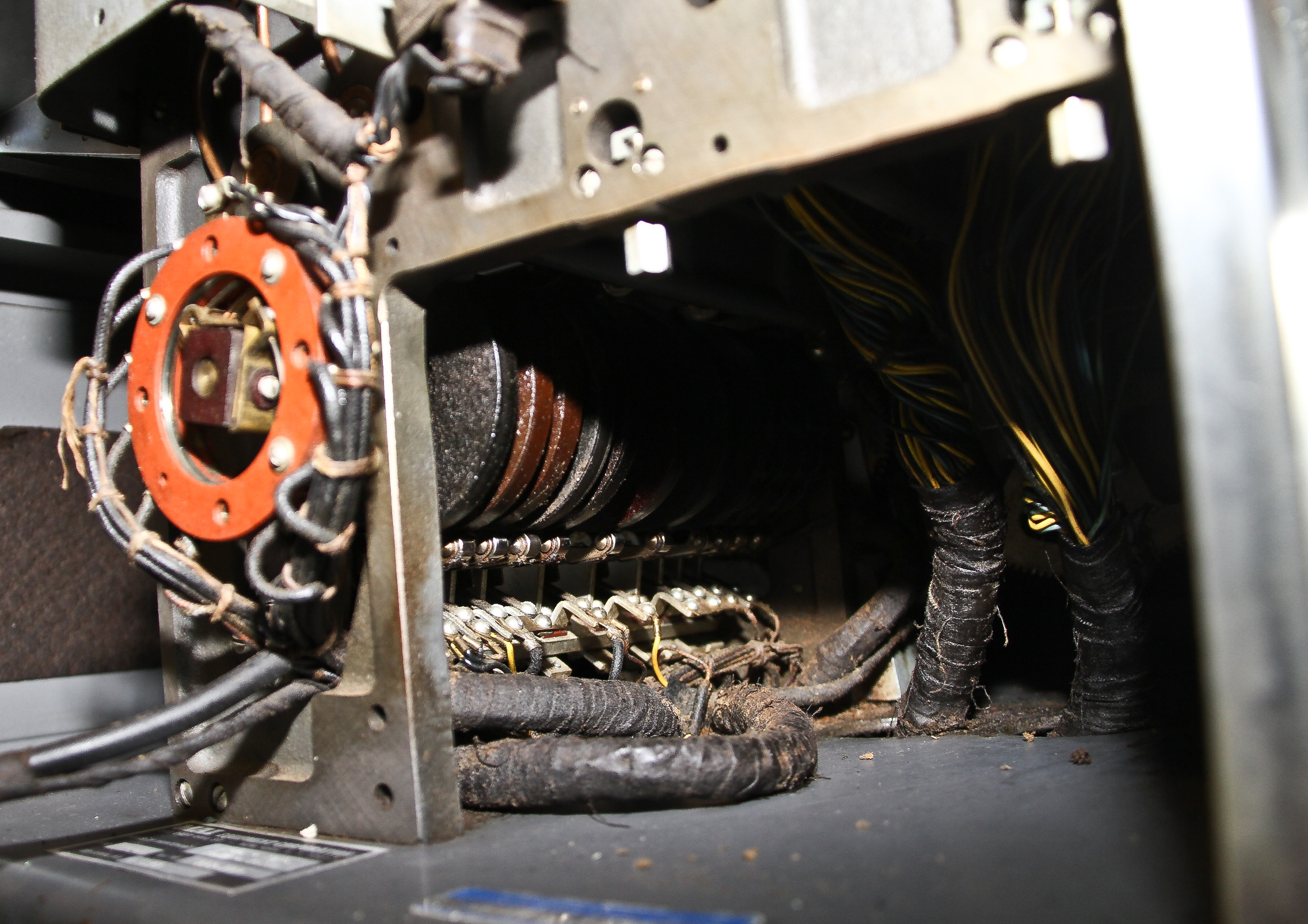
Figure 1 shows our IBM 514 Reproducing Punch. It basically reads punched cards and punches new cards based on the read cards, but not necessarily with the same data. In addition to simple punch-for-punch reproduction, based on the plugboard control the 514 can perform other functions such as inserting "master" information on each punched card, reproducing only some of the data and possibly in different locations, and creating and printing sequence numbers on the output cards.

Here is the quintessential piece of card equipment: a sorter. Our IBM 083 is one of the last of a line of IBM card sorters. Card sorters read one particular column as each card is passed through them and sends the card to the appropriate bin for what's punched in that column. Since there are 12 punch positions in each column, the read cards are routed one of 13 separate bins (12 plus one for errors). The 083 sorts at 1,000 cards a minute: over 16 per second. When it runs, it's very impressive; the cards move faster than the eye can follow. It also has a card counter for verifying the number of cards processed.


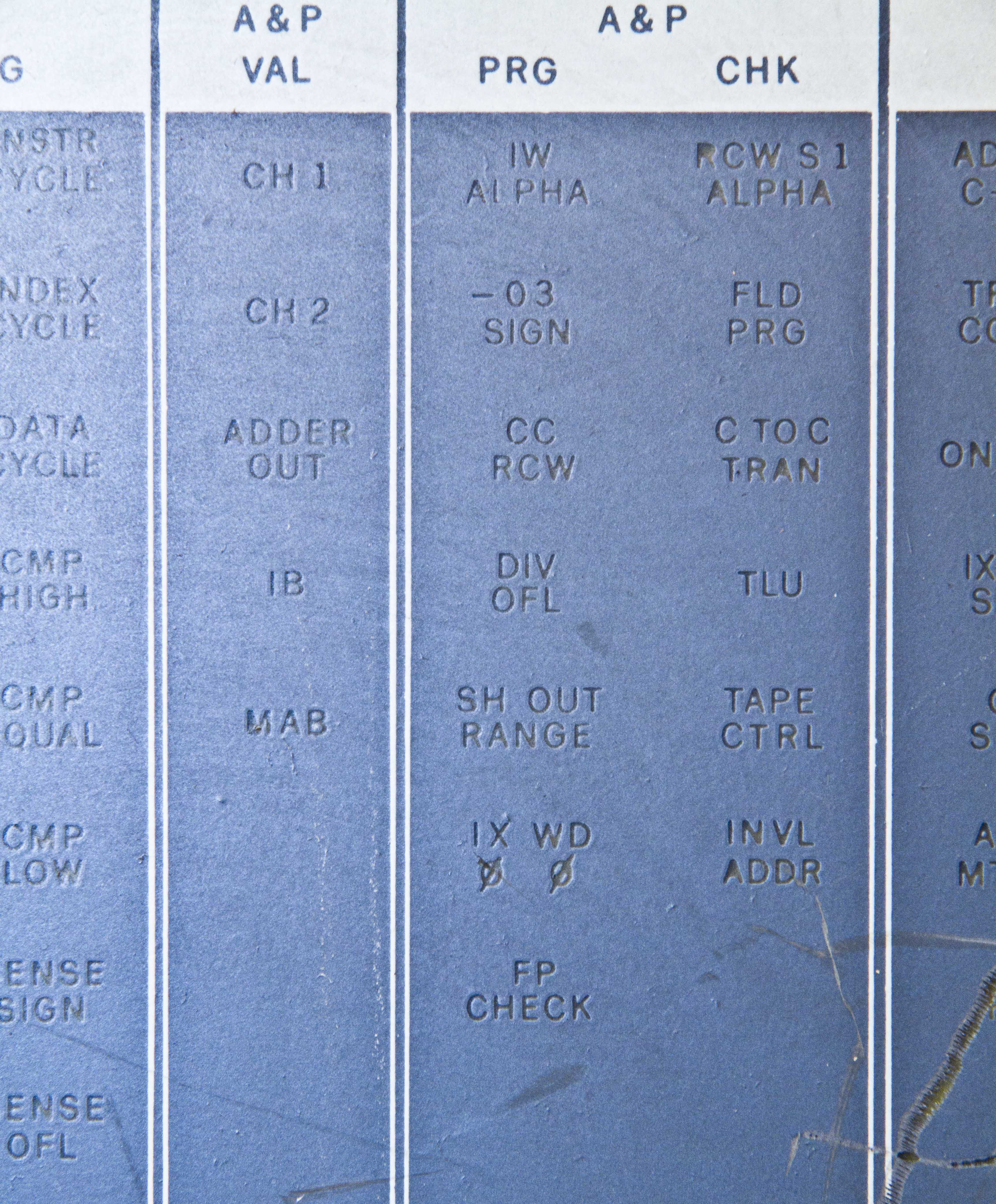
As mentioned elsewhere, the IBM System/360 family had a new and powerful type of I/O attachment: the IBM channel. The channel comprised a programmable I/O controller and standard physical attachments to a wide variety of I/O devices. There were two basic type of channel controllers: A selector channel, and a multiplexor channel.
The IBM 2870 was the multiplexor control unit for the System/360 family. Figure 1 is the control panel from an 2870 controller. (The wooden frame is an add-on for displaying the panel.) Figure 2 is a page from the 2870 manual showing this control panel. Careful study of the control and status indicators shows that the 2870 was effectively a programmable computer.